|
|
The U.S. Army Corps of Engineers HEC-RAS model (Version 5.0), under development since 1998,
can
perform the following five functions: (1)
one-dimensional steady flow, (2) one -dimensional unsteady flow,
(3) two-dimensional unsteady flow, (4) mobile-bed fluvial hydraulics, and
(5) water temperature and water quality modeling.
Here we compare the one-dimensional steady and unsteady flow modules.
The one-dimensional steady flow component
uses the standard step method for the solution of steady gradually varied flow.1
The one-dimensional unsteady flow component uses a
numerical solution of the equations governing gradually varied unsteady
flow in open channels.
When should unsteady flow be used?
This question is of considerable practical
interest, since unsteady flow is significantly more complex and requires more data than steady flow.
However, the answer is not straightforward, requiring some elaboration.
Steady vs unsteady flow
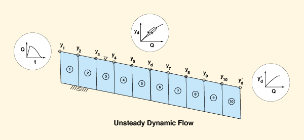
Under steady flow, the user inputs as boundary conditions a discharge upstream and a stage downstream.
The model proceeds to calculate stages throughout the interior points, keeping the discharge constant in space.
Under unsteady flow, the user inputs a discharge hydrograph at the upstream boundary and a discharge-stage rating
at the downstream boundary. The model calculates discharges and stages throughout the interior points.
Under steady flow, the calculated discharge-stage ratings are unique, i.e., kinematic.
On the other hand, under unsteady flow, the model calculates dynamic
looped discharge-stage
ratings according to the variabilities of the flow.
Therefore, the specification of a unique discharge-stage rating at the downstream boundary
contradicts the solution at that boundary.2
In essence, the model cannot be kinematic at the downstream
boundary and dynamic everywhere else.
A way out of the predicament is: (1) to artificially move the downstream boundary further downstream,
(2) to specify the unique discharge-stage rating at the
artificial downstream boundary, and (3) to let the model
calculate the looped ratings at the interior points,
including the point where the physical
downstream boundary is located.3 Despite its
apparent artificiality, this procedure works well,
circumventing the need to know the discharge-stage rating at the physical
downstream boundary before it is calculated.
Kinematic vs dynamic waves
The decision to use unsteady flow instead of steady flow
will depend on whether the wave to be modeled is construed as either kinematic
or dynamic.
If the wave is kinematic: (1) the discharge will not vary in space;
(2) the discharge-stage ratings will be unique; and (3) the downstream boundary may be specified as unique.
In this case, the solutions of steady and unsteady flow are essentially the same; therefore,
the unsteady flow calculation is not necessary.
If the wave is dynamic: (1) the discharge will vary in space, attenuating as it moves downstream, albeit
only for Froude numbers less than 2, which is usually the case;
(2) the calculated discharge-stage ratings
will not be unique; and (3) for better accuracy, the downstream boundary may be
artificially moved downstream to allow for an unsteady looped rating to develop
at the phyical downstream boundary.
In this case, the unsteady flow calculation is justified.
Use of unsteady flow in channel design
This situation begs the question of whether a certain flood wave can be construed as being either kinematic or dynamic.
Or, alternatively,
whether a dynamic wave should be used at all to determine stages in the design of channel improvement projects.
On typical projects, of limited channel lengths, a kinematic wave, which keeps its discharge constant,
is a better assumption than a dynamic wave, which attenuates its discharge. Indeed, the kinematic wave assumption assures that the
channel will contain all waves types,
kinematic, diffusion, and/or dynamic. Viewed in this light, the use of a dynamic wave for the calculation of stages in the
design of channel improvements projects does not appear to be warranted.
|
| 200520 07:30 |