|
| |
|
|
Muskingum-Cunge
amplitude and phase portraits
with online computation
Victor M. Ponce and Bavya Vuppalapati
30 April 2016
|
|
|
ABSTRACT
A comprehensive review of the amplitude and phase portraits of the Muskingum-Cunge method of flood routing is accomplished.
Expressions for the
amplitude and phase convergence ratios R1 and R2, respectively, are developed as a function of:
(a) spatial resolution L/Δx; (b) Courant number C; and (c) weighting factor X.
It is concluded that the Muskingum-Cunge routing model is a good representation of the physical prototype, provided:
(1) the spatial resolution is sufficiently high,
(2) the Courant number is close to 1, and
(3) the weighting factor is high enough, better if in the range 0.3 ≤ X ≤ 0.5.
Two online calculators of the convergence ratios, one theoretical based on dimensionless parameters, and the other practical, based on actual hydraulic/hydrologic variables,
are developed and tested.
|
1. INTRODUCTION
The concept of amplitude and phase portraits in computational hydraulics
is due to Leendertse (1967). The amplitude portrait is a plot of the ratio
of numerical to analytical wave amplitudes, i.e.,
a convergence ratio with regard to wave amplitude,
as a function of relevant variables such as the spatial
resolution or temporal resolution, and Courant number. Likewise,
the phase portrait is a plot of the ratio
of numerical to analytical wave celerities (a convergence ratio with regard to wave phase)
as a function of relevant numerical parameters. Amplitude and phase portraits
for the Muskingum-Cunge method of flood routing were originally developed by Cunge (1969), and later
expanded for the generalized convection (advection) problem by Ponce et al. (1979a).
The objective of amplitude and phase portraits are to
assess the stability and convergence
properties of a given numerical scheme. This helps determine
the range of discrete parameters (spatial resolution, temporal resolution, and their corresponding ratio)
for which the scheme may be shown to be stable and convergent. Following O'Brien et al. (1950),
stability is related to round-off errors, while convergence is related to
truncation (i.e., discretization) errors.
In this study, we revisit the amplitude and phase portraits of the Muskingum-Cunge method,
clarify their development, and further explain the details of the computation,
with aim to develop an online calculator.
2. MUSKINGUM-CUNGE METHOD
In a seminal paper,
Cunge (1969) elucidated the kinematic wave basis of the Muskingum method of flood routing (Chow, 1959),
leading to the Muskingum-Cunge method
(Natural Environment Research Council, 1975; Koussis, 1978; Ponce and Yevjevich, 1978).
Cunge's procedure allowed for the calculation of the weighting factor X in terms of physical
and numerical parameters, instead of relying solely on the
discharge, as proposed by the original Muskingum method (McCarthy, 1938).
This revolutionary concept, based on the matching of the physical diffusivity of
Hayami (1951) with the numerical
diffusivity of Cunge (1969), enables the Muskingum-Cunge method to remain grid independent through a wide
range of relevant parameters (spatial resolution, Courant number, and weighting factor). It is worth noting that this fundamental property
of the
Muskingum-Cunge method is not shared by other flood routing methods
based on the kinematic wave (Ponce, 1986).
In his original paper (op. cit.), Cunge expressed the amplitude and phase portraits in terms of the temporal resolution
and a type of Courant number.
Ponce et al. (1979b) expanded Cunge's approach to the
entire set of numerical schemes that can be construed to solve the general convection (advection)
equation. Ponce et al. (op. cit.) chose to present their findings for the amplitude and phase
convergence ratios in terms of the spatial resolution (L/Δx) and the
Courant number C, defined as the ratio of physical celerity c (i.e., the kinematic wave celerity) to numerical celerity
(the grid ratio Δx/Δt).
In this study, we review the findings of Ponce et al. (op. cit.) and apply them
specifically to the Muskingum-Cunge method.
3. DERIVATION OF EQUATIONS
The kinematic wave equation is (Cunge, 1969; Ponce, 2014a):
∂Q ∂Q
____ + c ____ = 0
∂t ∂x
| (1) |
in which Q = discharge, c = kinematic wave celerity, and x and t are space and time variables, respectively.
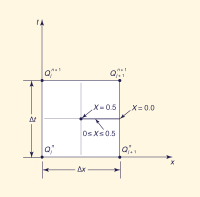
The discretization of Eq. 1 on the x-t plane (Fig. 1), assuming linearity (c = constant) leads to
(Ponce, 2014b):
X (Q j n+1 - Q j n ) + (1 - X) (Q j+1n+1 - Q j+1 n ) (Q j+1 n - Q j n ) + (Q j+1n+1 - Q
j n+1 )
________________________________________________ + c _______________________________________ = 0
Δt 2 Δx
| (2) |
Fig. 1 Space-time discretization of the kinematic wave equation
following the Muskingum-Cunge method.
Simplifying Eq. 2:
|
X (Q j n+1 - Q j n ) + (1 - X) (Q j+1n+1 - Q j+1 n ) + 0.5 C [ (Q j+1 n - Q j n ) + (Q j+1n+1 - Q
j n+1 ) ] = 0
| (3) |
in which C = Courant number, defined as follows:
The solution of Eq. 3 is postulated in the following exponential form (O'Brien et al., 1950; Cunge, 1969):
|
Q = Q* e i (σx - βt )
| (5) |
in which σ = (2π / L) is the wavenumber, L is the wave length, and β = (2 π / T )
is the wave period (Ponce and Simons, 1977).
Replacing Eq. 5 into the various components of Eq. 3:
|
Q j n = Q* e i [σj Δx - βn Δt ]
| (6) |
|
Q j+1n = Q* e i [σ (j + 1) Δx - βn Δt ]
| (7) |
|
Q j n+1 = Q* e i [σj Δx - β(n + 1) Δt ]
| (8) |
|
Q j+1n+1 = Q* e i [σj Δx - βn Δt ]
| (9) |
Equations 6 to 9 can be respectively expressed as follows:
e i σj Δx
Qj n = Q* ___________
e i βn Δt
| (10) |
e i σj Δx e i σΔx
Qj+1n = Q* _________________
e i βn Δt
| (11) |
e i σj Δx
Qj n+1 = Q* _________________
e i βn Δt e i βΔt
| (12) |
e i σj Δx e i σ Δx
Qj+1n+1 = Q* ___________________
e i βn Δt e i βΔt
| (13) |
The first term of Eq. 3 is:
e iσj Δx e iσj Δx
X (Q j n+1 - Q j n ) = Q* X [ _________________ - ___________ ]
e iβn Δt e iβΔt e iβnΔt
| (14a) |
e iσj Δx - e iσj Δx e iβΔt
X (Q j n+1 - Q j n ) = Q* X [ __________________________ ]
e iβn Δt e iβΔt
| (14b) |
The second term of Eq. 3 is:
e iσj Δx e iσΔx e iσj Δx e iσΔx
(1-X ) (Q j+1 n+1 - Q j+1 n ) = Q* (1 - X) [ __________________ - _________________ ]
e iβn Δt e iβΔt e iβnΔt
| (15a) |
e iσj Δx e iσΔx - e iβΔt e iσj Δx e iσΔx
(1-X ) (Q j+1 n+1 - Q j+1 n ) = Q* (1 - X) [ ________________________________________ ]
e iβn Δt e iβΔt
| (15b) |
The third term of Eq. 3 is:
|
(C / 2 ) (Q j+1n+1 - Q j n+1 + Q j+1n - Qj n ) =
| |
C Q* e iσj Δx e iσΔx - e iσjΔx + e iβΔt e iσj Δx e iσΔx - e iβΔt e iσj Δx
________ [ ___________________________________________________________ ]
2 e iβn Δt e iβΔt
| (16) |
Substituting Eqs. 14b, 15b, and 16 into Eq. 3,
dividing by Q* e iσj Δx, and eliminating the common denominator, leads to:
|
2X (1- e iβΔt ) + 2(1- X )(e iσΔx - e iσΔx e iβΔt ) + C (e iσΔx - 1 + e iβΔt e iσΔx - e iβΔt ) = 0
| (17a) |
|
e iβΔt [ -2X - 2(1-X ) e iσΔx + C e iσΔx - C ] + 2X + 2(1-X ) e iσΔx + C e iσΔx - C = 0
| (17b) |
|
e iβΔt [ 2X + 2(1-X )e iσΔx - C e iσΔx + C ] = 2X + 2(1-X ) e iσΔx + C e iσΔx - C
| (17c) |
2[X + (1-X ) e iσΔx] + C [e iσΔx - 1]
e iβΔt = ____________________________________
2[X + (1-X ) e iσΔx] - C [e iσΔx - 1]
| (17d) |
Rearranging Eq. 17d and taking the reciprocal value of the left-hand side:
2[(1-X) e iσΔx + X] - C [e iσΔx - 1]
e -iβΔt = ____________________________________
2[(1-X) e iσΔx + X] + C [e iσΔx - 1]
| (18) |
A trigonometric identity is (Spiegel, 1971):
in which
p = cos(σΔx) and q = sin(σΔx).
The spatial resolution is L /Δx.
The quantity
σΔx = (2π / L) Δx = 2π / (L/Δx)
is the number of grid points
per wavelength. Substituting Eq. 19 into Eq. 18:
2[(1-X)(p + iq) + X] - C [p + iq - 1]
e -iβΔt = _____________________________________
2[(1-X)(p + iq) + X] + C [p + iq - 1]
| (20a) |
{p [(1-X) - C/2] + X + C/2} + iq [(1-X) - C/2]
e -iβΔt = ______________________________________________
{p [(1-X) + C/2] + X - C/2} + iq [(1-X) + C/2]
| (20b) |
Defining for the sake of simplicity:
|
S = R - C = X - (C/2)
| (22) |
Substituting Eqs. 21 and 22 into Eq. 20b:
[p (1 - R) + R ] + iq (1 - R )
e -iβΔt = ______________________________
[p (1 - S) + S ] + iq (1 - S )
| (23) |
Multiplying the right-hand side of Eq. 23 by the conjugate of the denominator:
[p (1 - R) + R ] + iq (1 - R ) [p (1 - S) + S ] - iq (1 - S )
e -iβΔt = ______________________________ • ______________________________
[p (1 - S) + S ] + iq (1 - S ) [p (1 - S) + S ] - iq (1 - S )
| (24) |
{[p(1-R) + R ] [p(1-S) + S ] + q 2(1-R) (1-S)} + iq {(1-R) [p(1-S) + S ] - (1-S) [p(1-R) + R ]}
e -iβΔt = ____________________________________________________________________________________________
[ p (1-S )
+ S ] 2 + [ q (1-S )] 2
| (25) |
Now examine the components of Eq. 25. First consider the real part [RPN]
of the numerator of the right-hand side of Eq. 25:
|
[RPN] = [p (1-R) + R ] [p (1-S) + S ] + q 2(1-R ) (1-S )
| (26) |
Operating on Eq. 26, and after some algebraic manipulation:
|
[RPN] = 1 - (1-p) [R + S - 2RS]
| (27) |
Given that S = R - C, it follows that
R = S + C. Thus, in Eq. 27:
|
[RPN] = 1 - [ 2(1 - p)(1 - S)S ] - [ (1-p)(1 - 2S)C ]
| (28) |
Consider the imaginary part [IPN] of the numerator of Eq. 25:
|
[IPN] = q {(1-R ) [p (1-S ) + S ] - (1-S )[p (1-R ) + R ]}
| (29) |
Operating on Eq. 29, and after some algebraic manipulation:
Replacing R = S + C from Eq. 22 results in:
Consider the denominator [DN] of Eq. 25:
|
[DN] = [p (1-S ) + S ]2 + [q(1-S )]2
| (32) |
After some algebraic manipulation:
|
[DN] = 1 - 2 (1 - p)(1 - S) S
| (33) |
Defining for the sake of simplicity:
|
P = 1 - 2 (1 - p)(1 - S) S
| (34) |
Therefore, Eq. 25 can be written as follows:
P - M - iN
e -iβΔt = ______________
P
| (37a) |
which may be expressed as follows:
P - M N
e -iβΔt = _________ - i ______
P P
| (37b) |
In the left-hand side of Eq. 37b, separating β into its real and imaginary parts:
|
e -iβΔt = e -i (βR + i βI) Δt = e -i βR Δt e βI Δt
| (38a) |
|
e -iβΔt = e βI Δt e -i βR Δt = a eiφ
| (38b) |
in which a = e βI Δt, and eiφ = e i (-βR Δt)
In the right-hand side of Eq. 38a, taking the natural logarithm:
|
ln (e -i βR Δt e βI Δt) = ln e βI Δt - i βR Δt
| (39) |
Equation 37b can be expressed in the form z = x + iy, in which:
P - M
x = ________
P
| (41) |
The solution of Eq. 40 is (Spiegel, 1971):
|
ln(a eiφ) = ln (x2 + y2)1/2 + i tan-1(y / x)
| (43) |
Substituting Eqs. 38b, 41 and 42 into Eq. 43:
{(P - M)2 + N 2}1/2 N
ln e βI Δt - i βR Δt = ln [ ____________________ ] - i tan-1( _________ )
P P - M
| (44) |
Separating Eq. 44 into its real and imaginary components:
[(P - M)2 + N 2]1/2
e βI Δt = ____________________
P
| (45) |
N
tan (βR Δt) = _________
P - M
| (46) |
Since Eq. 1 does not allow for wave damping (eδ = 1, where δ = logarithmic decrement
(Ponce and Simons, 1977), it is concluded
that Eq. 45 is a measure of the numerical damping (- sign)
or amplification (+ sign) of the numerical solution of Eq. 3 after a time increment Δt.
4. CONVERGENCE RATIOS
Following Ponce et al. (1979c), a convergence ratio with regard to wave amplitude is:
Therefore:
[(P - M)2 + N 2]1/2
R1 = ____________________
P
| (48) |
The celerity of the numerical solution is:
Using Eqs. 46 and 49, a convergence ratio with regard to wave phase is defined as follows:
cn 1 N
R2 = _____ = ________ tan-1 ( _________ )
c σ c Δt P - M
| (50) |
in which cn is the wave celerity of the numerical solution, c is the kinematic wave celerity (in Eq. 1), and σ is the wavenumber.
From Eq. 4: C Δx = c Δ t. Therefore:
1 N
R2 = _________ tan-1 ( ________ )
C σΔx P - M
| (51) |
In summary, given only: -
Weighting factor X,
- Spatial resolution L/Δx, from which: σΔx
= (2π /L) Δx = 2 π / (L /Δx),
and
- Courant number C,
Equations 48 and 51 enable the calculation of the Muskingum-Cunge amplitude and phase
convergence ratios, respectively.
The calculation of the convergence ratios is accomplished
using the calculator
Online Muskingum-Cunge Convergence Ratios.
5. AMPLITUDE AND PHASE PORTRAITS
The plotting of convergence ratios R1 and
R2 as a function of Courant number C and spatial resolution L/Δx
leads to a set of amplitude and phase portraits, a pair for each value of
weighting factor X.
Figures 2 to 8 show the amplitude and phase portraits of the Muskingum-Cunge method (Eq. 3),
for Courant numbers varying in the range
0.1 ≤ C ≤ 4.0, spatial resolution 20 ≤ L/Δx ≤ 100, at intervals of L/Δx = 20,
and weighting factor 0.0 ≤ X ≤ 0.6, at intervals of X = 0.1 (7 × 2 = 14 graphs).
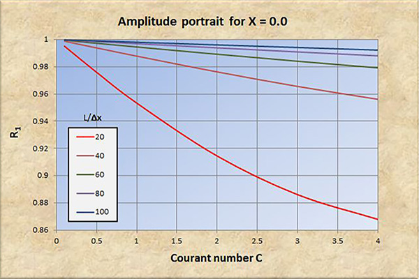
Fig. 2 (a) Amplitude portrait for X = 0.
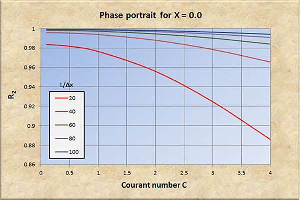
Fig. 2 (b) Phase portrait for X = 0.
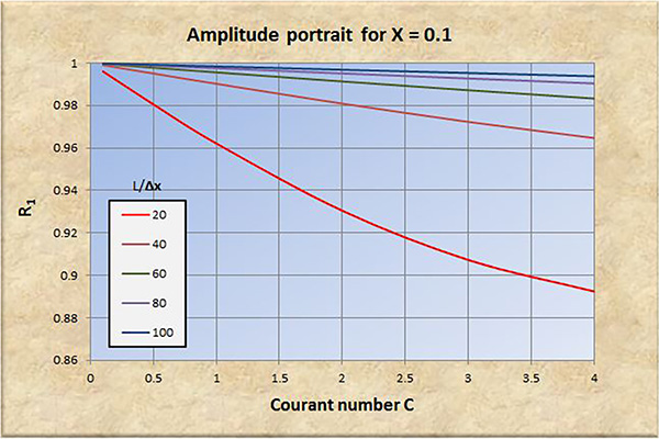
Fig. 3 (a) Amplitude portrait for X = 0.1.
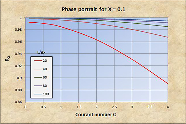
Fig. 3 (b) Phase portrait for X = 0.1.
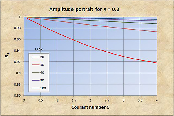
Fig. 4 (a) Amplitude portrait for X = 0.2.
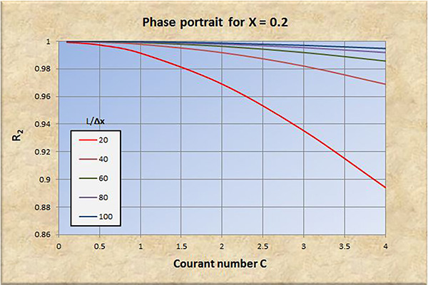
Fig. 4 (b) Phase portrait for X = 0.2.
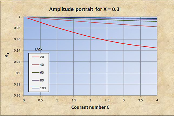
Fig. 5 (a) Amplitude portrait for X = 0.3.
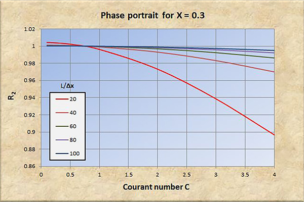
Fig. 5 (b) Phase portrait for X = 0.3.
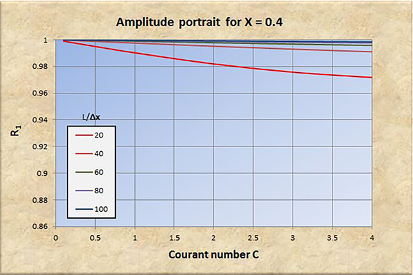
Fig. 6 (a) Amplitude portrait for X = 0.4.

Fig. 6 (b) Phase portrait for X = 0.4.
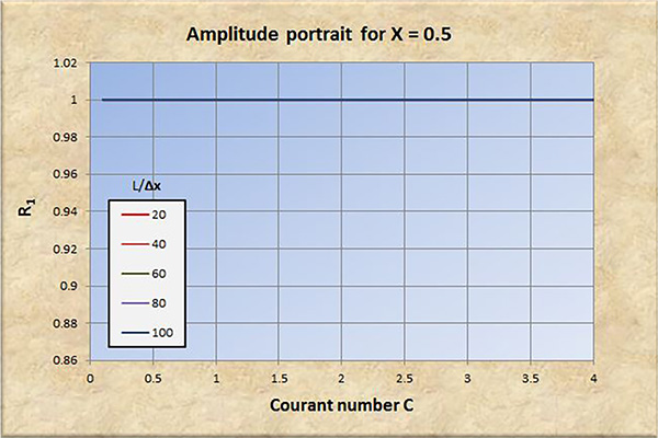
Fig. 7 (a) Amplitude portrait for X = 0.5.
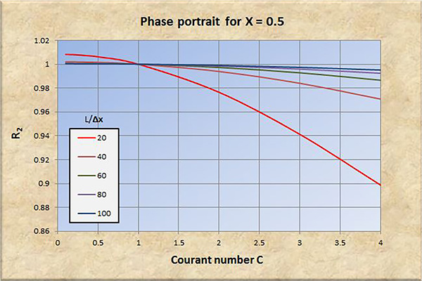
Fig. 7 (b) Phase portrait for X = 0.5.
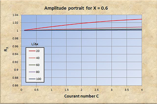
Fig. 8 (a) Amplitude portrait for X = 0.6.

Fig. 8 (b) Phase portrait for X = 0.6.
6. ANALYSIS
The examination of Figs. 2 to 8 leads to the following conclusions:
Perfect convergence is achieved for X = 0.5 and Courant number C = 1.
Convergence in both amplitude and phase improves with an increase in spatial resolution (L/Δx).
Convergence in both amplitude and phase degrades with an increase in Courant number C, particularly for C > 1.
Convergence in amplitude improves with an increase in X in the range 0 ≤ X ≤ 0.5.
Convergence in phase improves slightly with an increase in X in the range 0 ≤ X ≤ 0.5.
At low spatial resolutions [refer to red curves in Figs. 2 (b) to 8 (b)], convergence in phase degrades significantly with Courant numbers in the range C < 1, leading to instability.
For X > 0.5, the amplitude convergence
ratio R1 becomes positive (amplification), and convergence and stability degrade accordingly.
We conclude that the Muskingum-Cunge model is a good representation of the physical prototype, provided:
The spatial resolution is sufficiently high.
The Courant number is close to 1.
The weighting factor is high enough, in the range 0.0 ≤ X ≤ 0.5.
Based on the analysis accomplished herein, the recommended parameter values for adequate convergence are: (a) spatial resolution L/Δx ≥ 100; (b) Courant number C ≅ 1; and (c) weighting factor 0.3 ≤ X ≤ 0.5.
7. PRACTICAL APPLICATIONS
In practical applications, the convergence of the Muskingum-Cunge method depends on the values of Courant and cell Reynolds numbers, which in turn,
depend on the hydraulics of the flow and the grid size (Δx and Δt) (Ponce, 2014c).
A set of amplitude and phase convergence ratios may be calculated
in terms of hydraulic and hydrologic variables.
To this end, define the time-of-rise tr of the flood wave as the time it takes for the flood wave to reach the peak flow.
Assuming a sinusoidal perturbation as a first approximation, the time base, or wave period T is:
The wave celerity c is:
in which u is the mean flow velocity.
In turbulent
open-channel flow, the value of β
varies from β = 5/3 for a hydraulically wide channel, down to β = 1 for
an inherently stable channel (Ponce and Porras, 1995;
Ponce, 2014d).
The wavelength L of the perturbation is:
The unit-width discharge q is:
in which d is the mean flow depth. The spatial resolution is L/Δx.
The Courant number (Eq. 4), repeated here with a new equation number, is:
The cell Reynolds number is defined as follows ((Ponce, 2014e):
q
D = ___________
So c Δx
| (57) |
By definition, the Muskingum-Cunge weighting factor X is:
1
X = ____ (1 - D)
2
| (58) |
For a given case, Eqs. 52 to 58, together with Eqs. 48 and 51, enable the calculation
of the practical convergence ratios of the Muskingum-Cunge method,
based on actual flow data, i.e., on the hydraulics of the flow.
The calculation of the Muskingum-Cunge practical convergence ratios may be accomplished
using the calculator
Online Muskingum-Cunge Convergence Ratios Practical.
For example, assume the following data set: (1) mean velocity u = 1.75 m/s; (2) mean flow depth d = 2.3 m;
(3) mean channel slope S = 0.0013; rating exponent β = 1.6, (5) flood wave time-of-rise tr = 24 hr;
(6) reach length Δx = 4,800 m, and (7) time interval Δt = 0.5 hr. The application of
Online Muskingum-Cunge Convergence Ratios Practical leads to: R1 = 0.99953; R2 = 0.999915.
In this case, the spatial resolution is L/Δx = 100.8; the Courant number is C = 1.05; and the weighting factor is X =
0.385. All three parameters lie within the recommended ranges for adequate convergence.
8. CONCLUSIONS
A comprehensive review of the Muskingum-Cunge method's amplitude and phase portraits is accomplished.
Expressions for the
amplitude convergence ratio R1 and phase convergence ratio R2 are developed as a function of:
(a) spatial resolution L/Δx; (b) Courant number C; and (c) weighting factor X.
An online calculator
Online Muskingum-Cunge Convergence Ratios is developed and tested using a realistic data set.
In practical applications, the convergence ratios may be expressed alternatively in terms of
relevant hydraulic variables (mean velocity, flow depth, channel slope, rating exponent,
and flood wave time-of-rise). For this case, an online calculator
Online Muskingum-Cunge Convergence Ratios Practical is also developed and tested.
REFERENCES
Chow, V. T. 1959. Open-channel hydraulics. McGraw-Hill, New York.
Cunge, J. A.. 1969.
On the subject of a flood propagation computation method (Muskingum method). Journal of Hydraulic Research, Vol. 7, No. 2, 205-230.
Hayami, S. 1951. On the propagation of flood waves. Bulletin No. 1, Disaster Prevention Research Institute,
Kyoto University, Kyoto, Japan, December.
Koussis, A. 1978. Theoretical estimation of flood routing parameters. Journal of the Hydraulics Division, ASCE,
Vol. 104, No. HY1, Proc. Paper 13456, January, 109-115.
Leendertse, J. J. 1967. Aspects of a computational model for long-period water wave propagation. Report RM-5294-PR, The Rand Corporation,
Santa Monica, California, May.
McCarthy, G. T. 1938. The unit hydrograph and flood routing. Unpublished manuscript, presented at a conference of the North Atlantic Division,
U.S. Army Corps of Engineers, June 24, 1938.
Natural Environment Research Council. 1975. Flood Studies Report, Vol. III: Flood Routing Studies, London, England.
O'Brien, G. G., M. A. Hyman, and S. Kaplan. 1950. A study of the numerical solution of partial differential equations.
Journal of Mathematics
and Physics, Vol. 29, No. 4, 223-251.
Ponce, V. M., and D. B. Simons. 1977. Shallow wave propagation in open channel flow.
Journal of the Hydraulics Division, ASCE, Vol. 103, No. HY12, December, 1461-1476.
Ponce, V. M., and V. Yevjevich. 1978.
Muskingum-Cunge method with variable parameters.
Journal of the Hydraulics Division, ASCE, Vol. 104, No. HY12, December, 1663-1667.
Ponce, V. M., Y. H. Chen, and D. B. Simons. 1979. Unconditional stability in convection computations. Journal of the Hydraulics Division, ASCE, Vol. 105, No. HY9, September, 1079-1086.
Ponce, V. M. 1986. Diffusion wave modeling of catchment dynamics.
Journal of Hydraulic Engineering, ASCE, Vol. 112, No. 8, August, 716-727.
Ponce, V. M., and P. J. Porras. 1995. Effect of cross-sectional shape on free-surface instability. Journal of Hydraulic Engineering, ASCE, Vol. 121, No. 4,
April, 376-380.
Ponce, V. M. 2014. Fundamentals of open-channel hydraulics.
Online text.
Spiegel, M. R. 1971. Advanced mathematics for engineers and scientists. Schaum's Outline Series, McGraw-Hill Inc., New York.
|