|
ABSTRACT
The propagation characteristics of various types of shallow water waves in open channel flow are calculated on the basis of linear stability theory. The celerity and attenuation functions of kinematic, diffusion, convective dynamic, dynamic and gravity waves, are derived. For the most general case, i.e., the dynamic wave model, the propagation characteristics are expressed as a function of the steady uniform flow Froude number and the dimensionless wave number of the unsteady component of the motion. The wave number spectrum is divided into three bands: (1) A gravity band corresponding to large wave number, where the wave celerity is the gravity wave celerity; (2) a kinematic band corresponding to a small wave number where the wave celerity is the kinematic wave celerity; and (3) a dynamic band corresponding to mid-spectrum values of the wave number, where the wave celerity falls between the gravity and kinematic celerity values.
|
1. INTRODUCTION
Over the years, several investigators have attempted to clarify the phenomenon of propagation of shallow waves in open channel flow. Perhaps the most illuminating of these studies is that reported in the classical paper by Lighthill and Whitham, which analyzed in detail the concept of kinematic wave and contrasted it to the dynamic wave (5). The Lagrange formula for the celerity of shallow gravity waves has also been a subject of considerable attention in the literature (3). Despite the progress made in the understanding of the physical phenomenon, a coherent theory that accounts for celerity as well as attenuation characteristics has yet to be formulated. In this respect, the theory of linear stability can be used as an effective tool, not only to furnish a first approximation analysis, but also to provide valuable insight into the underlying physics of the problem (6).
The analysis presented herein endeavors to apply the theory of linear stability to the set of equations governing the motion in open channel flow. The equations are the so-called Saint Venant equations, which are analytical expressions of the principle of mass and momentum conservation (1). The conclusions relate to the magnitude of celerity and attenuation of various types of shallow water waves, expressed as a function of the Froude number of the steady uniform flow and a dimensionless wave number of the unsteady component of the motion.
2. GOVERNING EQUATIONS
The governing equations for the one-dimensional unsteady flow in broad channels of rectangular cross section, expressed per unit of channel width, are the equation of continuity (4):
∂d ∂u ∂d
u ____ + d ____ + ____ = 0
∂x ∂x ∂t
| (1) |
and the equation of motion:
1 ∂u u ∂u ∂d
____ _____
+ ____ _____ + _____ + (Sf - So ) = 0
g ∂t g ∂x ∂x
| (2) |
in which u = velocity averaged in a vertical section, d = depth of flow; g = acceleration of gravity; Sf = friction slope; and So = bed slope.
The friction slope Sf is directly related to the bottom shear stress τ
by the expression (2):
in which γ = unit weight of water.
In the usual manner of stability calculations, Eqs. 1 and 2 must satisfy the unperturbed flow for which u = uo; d = do; and τ = τo, as well as the perturbed flow for which u = uo + u' ; d = do + d' ; and τ = τo + τ' (7).
The superscript in the flow variables represents a small perturbation to the steady uniform flow. Thus, all quadratic terms in the fluctuating components may be neglected based on an order of magnitude reasoning.
Substitution of the perturbed variables in Eqs. 1, 2, and 3 yields, after linearization (5):
∂d' ∂u' ∂d'
uo ____ + do ____ + ____ = 0
∂x ∂x ∂t
| (4) |
1 ∂u' uo ∂u' ∂d' τ' d'
____ _____
+ ____ _____ + _____ +
So ( _____ - _____ ) = 0
g ∂t g ∂x ∂x τo do
| (5) |
in which:
The boundary shear stress τ may be related to the mean velocity as follows:
in which:
where Cf = Chezy coefficient; and ρ = the density of water. Considering Eq. 7, Eq. 5 can be rewritten as follows:
1 ∂u' uo ∂u' ∂d' u' d'
____ _____
+ ____ _____ + _____ +
So ( 2 _____ - _____ ) = 0
g ∂t g ∂x ∂x uo do
| (9) |
For most practical applications, the Manning equation is preferred over the Chezy equation. The latter, however, has the advantage of nondimensionality, and it is for this reason that it is used here. Furthermore, the constant Cf is consistent with the small perturbation assumption.
3. WAVE MODELS
The propagation of shallow water waves is controlled by the balance of the
various forces included in the equation of motion. In Eq. 2, the first term
represents the local inertia term, the second term represents the convective
inertia term, the third term represents the pressure differential term, and the
fourth accounts for the friction and bed slopes. Various wave models may be
construed, depending on which of these four terms is assumed negligible when
compared with the remaining terms.
The following chart provides a ready reference to the various wave models that are recognized.
Term I II III IV
Equation 1 ∂u u ∂u ∂d
of motion ____ _____
+ ____ _____ + _____ + (Sf - So ) = 0
g ∂t g ∂x ∂x
| (2) |
Wave model and terms used to describe it are: (I) kinematic wave IV; (2) diffusion wave III + IV; (3) steady dynamic wave II + III + IV; (4) dynamic wave I + II + III + IV; and (5) gravity wave I + II + III.
4. SMALL PERTURBATION ANALYSIS
In order to provide for a convenient way to take explicit account of the various wave models, Eq. 9 is recast as follows:
l ∂u' auo ∂u' ∂d' u' d'
____ _____
+ _____ _____ + p _____ +
k So ( 2 _____ - _____ ) = 0
g ∂t g ∂x ∂x uo do
| (10) |
in which l, a, p, and k are integers that can take values of 0 and 1 only, depending on which terms of Eq. 9 are used to describe the motion.
The solution for a small perturbation in the depth of flow is postulated in the following exponential form:
d'
____ = d* e i (σ* x* - β* t* )
do
| (11) |
in which d' is a small perturbation to do; d* is a dimensionless depth amplitude
function; σ* is a dimensionless wave number β* is a dimensionless complex propagation factor, and x* and t* are dimensionless space and time coordinates such that:
2 π
σ* = (
_____ ) Lo
L
| (12) |
2 π Lo
β*R = (
_____ ) _____
T uo
| (13) |
|
β* I = amplitude propagation factor
| (14) |
in which L = wavelength of the disturbance; and T = period. The value Lo = the horizontal length in which the steady uniform flow drops a head equal to its
depth, defined as Lo = do/So.
The dimensionless celerity of the disturbance is given by the following:
L / T β*R
c* =
________ = _______
uo σ*
| (17) |
The wave attenuation follows an exponential law in which the amplitude at a given time t = the initial amplitude at time to multiplied by (e β*I t* ), in which t* = (t - to) uo / Lo. When comparing wave amplitudes after one propagation period, the value of t* is t* = T uo / Lo, or likewise, t* = 2 π / |β*R|. The logarithmic decrement δ is defined as δ = β* T u o / Lo, or δ = 2 π β*I / |β*R| (10). The value of δ is a measure of the rate at which the unsteady component of the motion changes upon propagation. For δ positive, amplification sets in; for δ negative, the motion attenuates and dies away.
The depth disturbance is associated with a velocity disturbance of the following form:
u'
____ = u* e i (σ* x* - β* t* )
uo
| (18) |
in which u* is a dimensionless velocity amplitude function. The substitution of Eqs. 11 and 18 into Eqs. 4 and 10 yields, respectively:
σ* u*
+ (σ* - β* ) d* = 0
| (19) |
[ 2k + i Fo2 (α σ* -
l β* ) ] u*
+ (i p σ* - k ) d* = 0
| (20) |
in which:
uo 2
Fo2 = ______
g do
| (21) |
Equations 19 and 20 constitute a homogeneous system of linear equations in the unknowns u* and d*. For the solution to be nontrivial, the determinant of the coefficient matrix must vanish. Accordingly:
i l β* 2 Fo2 - i
σ*2 (p - a Fo2 ) + 3 k σ* -
2 k β* - i σ* β* (l + a) Fo2 = 0
| (22) |
Equation 22 is the characteristic equation governing the propagation of small amplitude water waves. In the treatment that follows, successive simplifications will be made to conform to the various types of wave models considered in the previous section.
5. KINEMATIC WAVE MODEL
In the kinematic wave model, the inertia and pressure terms are negligible as compared to the friction-bed slope term.
Accordingly, in Eq. 22, l = a = p = 0; and k = 1, resulting in the following:
Since all the imaginary terms have dropped out in Eq. 23, β*I = 0; and β*R = β*. The logarithmic decrement δk , is then:
β*I
δk = 2π
_____ = 0
β*R
| (24) |
and the dimensionless celerity of the kinematic wave is:
β*R 3
c* k = _____ = ____
T 2
| (25) |
Equations 23 to 25 warrant the following conclusions regarding kinematic wave propagation: (1) Since Eq. 23 is of the first order, kinematic waves propagate only in the downstream direction; (2) the celerity of a kinematic wave is independent of Fo and σ* and equal to 1.5 times the mean flow velocity; and (3) the attenuation of a kinematic wave is zero, i.e., a kinematic wave propagates downstream without dissipation.
6. DIFFUSION WAVE MODEL
In the diffusion wave model, the inertia terms are considered negligible, but the pressure term is taken into account. Accordingly, in Eq. 22, l = a = 0; p = k = 1, resulting in the following:
|
- i σ* 2 + 3 σ* - 2 β* = 0
| (26) |
and
3 σ* - i σ* 2
β* =
______________
2
| (27) |
and the celerity of the diffusion wave is:
β*R 3
c*d = _____ = _____
σ* 2
| (28) |
The logarithmic decrement is:
β*I σ*
δd = 2 π ______ =
- 2 π ( ____ )
β*R 3
| (29) |
The following conclusions are derived for diffusion waves: (1) Because Eq. 26 is of first order in β*, diffusion waves propagate downstream only, and their celerity is independent of Fo and σ*, and equal to 1.5 the mean flow velocity; and (2) diffusion waves attenuate as they propagate downstream, and the rate of attenuation is controlled by the dimensionless wave number σ*. The larger the dimensionless wave number, the greater the attenuation.
7. STEADY DYNAMIC WAVE MODEL
In the steady dynamic wave model, the convective inertia term is brought into the problem, and the local inertia term is neglected. Accordingly, in Eq.
22, l = 0; and a = p = k = 1, resulting in:
|
- i σ* 2 (1 - Fo2 ) + 3 σ* - 2 β* - i σ* β* Fo2 = 0
| (30) |
and
3 σ* - i σ*2 ( 1 - Fo2 )
β*
= _______________________
2 + i σ* Fo2
| (31) |
or
σ* [ 6 - σ*2 Fo2 ( 1 - Fo2 )] - i σ*2 ( 2 + Fo2 )
β*
= ___________________________________________
4 + σ*2 Fo4
| (32) |
From Eq. 32, the celerity of the steady dynamic model is:
2 - σ* 2 Fo2
c*s
= 1 + ______________
4 + σ*2 Fo4
| (33) |
The logarithmic decrement is:
σ* ( 2 + Fo2 )
δs
= - 2 π ________________________
| 6 - σ*2 Fo2 ( 1 - Fo2 ) |
| (34) |
The following conclusions are derived regarding the steady dynamic model: (1) The propagation of the steady dynamic wave is in one direction, since Eq. 30 is of first order in β*; and (2) the celerity and attenuation characteristics are functions of the Froude number of the steady uniform flow Fo and the dimensionless wave number σ*.
8. DYNAMIC WAVE MODEL
In the dynamic wave model, all terms in the equation of motion are considered.
Thus, in Eq. 22, l = a = p = k = 1. It follows that:
Fo2 β*2 - 2 ( σ* Fo2 - i ) β* - [ σ*2 ( 1 - Fo2 ) + 3 σ* i ] = 0
| (35) |
Equation 35 is of the second order, resulting in two roots. Physically speaking, dynamic waves propagate along two characteristic paths, which can face either: (1) one upstream and another downstream; or (2) both downstream. In the case of propagation in different directions, it is expedient to define as primary wave the wave that travels downstream, and identify its celerity and logarithmic decrement by c*1 and δ1, respectively. The secondary wave is defined as the wave traveling upstream with celerity c*2 and logarithmic decrement δ2. In the case of both waves traveling downstream, primary wave is the faster wave, and secondary wave is the slower wave.
The solution of Eq. 35 is the following:
1
β* =
σ* ( 1 - i ζ ) + σ* [ ( ______ - ζ 2 ) + i ζ ] 1/2
Fo2
| (36) |
in which:
1
ζ =
_________
σ* Fo2
| (37) |
An expression of the same type as Eq. 37 is referred to in the literature as kinematic flow number (9).
The complex square root argument can be expressed in polar form as follows:
A + i B = C ( cos θ + i sin θ )
| (38) |
in which:
1
A =
______ - ζ 2
Fo2
| (39) |
1
C = [ (
______ - ζ 2 ) 2 + ζ 2 ] 1/2
Fo2
| (41) |
and the root of the complex argument is:
θ + 2 k π θ + 2 k π
(A + i B )1/2 = C1/2 ( cos __________ + i sin ___________ ) ; for k = 0,1
2 2
| (43) |
and by use the half-angle relations:
1 + cos θ 1 - cos θ
(A + i B )1/2 = ± C1/2 [ ( __________ )1/2 + i ( __________ )1/2 ]
2 2
| (44) |
in which use has been made of the fact that because ζ ≥ 0, θ/2 falls in the first quadrant.
Since:
it follows that:
C + A C - A
(A + i B )1/2 = ± [ ( ________ )1/2 + i ( ________ )1/2 ]
2 2
| (46) |
or
C + A C - A
β* = σ* (1 - i ζ ) ± σ* [ ( ________ )1/2 + i ( ________ )1/2 ]
2 2
| (47) |
From Eq. 47, the following two roots are obtained:
C + A C - A
β*1 = σ* [ 1 + ( ________ )1/2 ] - i σ* [ ζ - ( ________ )1/2 ]
2 2
| (48) |
C + A C - A
β*2 = σ* [ 1 - ( ________ )1/2 ] - i σ* [ ζ + ( ________ )1/2 ]
2 2
| (49) |
Now call:
C + A
D = (
_________ ) 1/2
2
| (50) |
and
C - A
E = (
_________ ) 1/2
2
| (51) |
and the celerity and attenuation functions are given by:
For the primary wave:
C + A
c*1 = 1 + (__________ ) 1/2
2
| (52) |
ζ - E
δ1 = - 2π _____________
| 1 + D |
| (53) |
For the secondary wave:
C + A
c* 2 = 1 - (
_________ ) 1/2
2
| (54) |
ζ + E
δ2 = - 2π ___________
| 1 - D |
| (55) |
| TABLE 1. Propagation characteristics of shallow water waves in open channel flow.
|
Type of wave
(1) | Relative celerity c*r
(2) | Logarithmic decrement δ
(3) |
| Kinematic |
1/2 |
0 |
| Diffusion |
1/2
|
- 2 π ( σ* / 3 ) |
| Steady dynamic |
( 2 - σ*2 Fo2 ) / ( 4 + σ*2 Fo4 ) |
- 2 π σ* ( 2 + Fo2 ) / | 6 - σ*2 Fo2 ( 1 - Fo2 ) | |
| (a) Dynamic
|
| Primary wave |
+ [(C + A ) / 2 ] 1/2 |
- 2 π ( ζ - E ) / | 1 + D | |
| Secondary wave |
- [(C + A ) / 2 ] 1/2 |
- 2 π ( ζ + E ) / | 1 - D | |
| (b) Gravity
|
| Primary wave |
+ 1 / Fo |
0 |
| Secondary wave |
- 1 / Fo |
0 |
Note: ζ = 1 / ( σ* Fo2 ) ; A = ( 1 / Fo2 ) - ζ 2 ; C = { [ ( 1 / Fo2 ) - ζ 2 ] 2 + ζ 2 } 1/2 ; D = [ (C + A ) / 2 ] 1/2 ;
E = [ (C - A ) / 2 ] 1/2 .
|
|
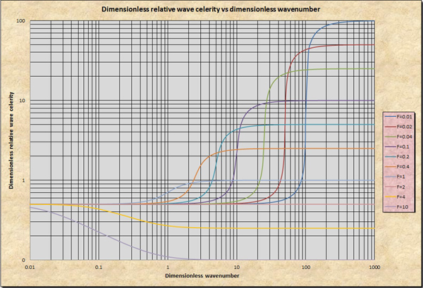
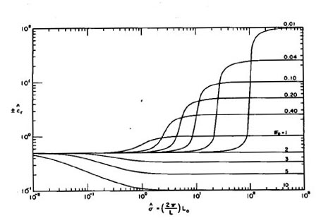
Fig. 1 Dimensionless relative celerity c*r vs dimensionless wave number σ*;
curve parameter = Froude number Fo (0.01 ≤ Fo ≤ 10).
|
|
9. GRAVITY WAVE MODEL
In the gravity wave model, the friction and bed slope terms are excluded from the momentum equation. It follows that, in Eq. 22, l =�a = p = 1; and k = 0, resulting in:
|
β*2 Fo 2 - 2 σ* β* Fo 2 - σ* 2 (1 - Fo 2 ) = 0
| (56) |
Since Eq. 56 is of the second order in β* and contains no imaginary terms, gravity waves have two characteristic directions and are not subject to attenuation.
Solving for β*R in Eq. 56:
Fo 2 ± Fo
β*R = σ* (
___________ )
Fo 2
| (57) |
and the celerity of a gravity wave is given as follows:
β*R 1
c* g = _____ = 1 ± _____
σ* Fo
| (58) |
or in the more usual way of expressing it (Lagrange formula):
|
cg = uo ± ( g do )1/2
| (59) |
Gravity waves propagate along two characteristic directions. In subcritical flow, one direction is downstream. with celerity c1 = uo + (g do)1/2, and another is upstream, with celerity c2 = uo - (g do)1/2. In critical flow, c1 = 2uo; and c2 = 0. In supercritical flow, both waves travel downstream, with celerities c1 = uo + (g do)1/2; and c2 = uo - (g do)1/2.
A summary of the propagation characteristics of the various waves described is given in Table 1. The celerity shown in Table 1 is the relative celerity c* r , in which:
10. ANALYSIS OF THE DYNAMIC MODEL
Equations 52-55 enable the calculation of the propagation characteristics of the dynamic wave model, as a function of the Froude number Fo of the steady uniform flow and the dimensionless wave number σ* of the sinusoidal perturbation superimposed on the steady uniform flow.
Figure 1 shows the calculated values of the dimensionless relative celerity c*r versus the dimensionless wave number σ* for Froude numbers between 0.01-10. The following conclusions are derived from this figure:
There are three well-defined bands in the wave number spectrum: (a) a kinematic band corresponding to small values of the wave number σ*, in which the relative celerity c*r is independent of both σ* and the Froude number Fo; (b) a gravity band corresponding to large values of σ*, in which c*r is independent of σ* and dependent only on Fo ; and (c) a dynamic band, in which c*r is a function of both σ* and Fo.
In the kinematic band, c*r approaches asymptotically a constant value of 0.5, which corresponds to that of a kinematic wave. In the gravity band, c*r approaches asymptotically the value 1/Fo, which corresponds to that of a gravity wave. In the dynamic band, c*r lies between the kinematic and gravity wave celerity values.
The location of the dynamic band in the σ* spectrum is a function of Fo.
A corollary resulting from Fig. 1 is that for Fo = 2, c*r = 0.5 for all values of σ*. Thus, at Fo = 2, all waves, kinematic, dynamic, and gravity, have celerities equal to the kinematic value. The conclusions of Fig. 1 regarding the limiting value of c*r , in the kinematic and gravity bands can be obtained analytically based on limit theory. It can be shown that as σ* → ∞ , c*r → 1/Fo , and as σ* → 0, c*r → 0.5 (for Fo constant).
The calculation of the logarithmic decrements
δ1 and δ2 as a function of σ* and Fo, by means of Eqs. 53 and 55 enable the following general conclusions:
For Fo < 2, primary waves propagate downstream and attenuate; for Fo = 2, primary waves propagate downstream and neither amplify nor attenuate
throughout the σ* spectrum; for Fo > 2 primary waves propagate downstream and amplify.
For Fo < 1, secondary waves propagate upstream (c*r > 1), or downstream (c*r < 1). For F = 1, secondary waves remain stationary (c*r = 1), or propagate downstream (cr < 1). For Fo > 1, secondary waves propagate downstream. Secondary waves attenuate for all Fo and σ*.
Table 2 summarizes the conclusions of the foregoing paragraph.
| TABLE 2. Celeritya and attenuationb characteristics of the dynamic wave. |
Froude number
(1)
| Primary Wave
| Secondary Wave
|
c*1
(2)
| δ1
(3)
| c*2
(4)
| δ2
(5)
|
| Fo < 1
| +
| -
| -
| -
|
| +
| -
|
| Fo = 1
| +
| -
| 0
| -
|
| +
| -
|
| 1 < Fo < 2
| +
| -
| +
| -
|
| Fo = 2
| +
| 0
| +
| -
|
| Fo > 2
| +
| +
| +
| -
|
a Downstream celerity + ; upstream celerity -.
b Attenuation - ; amplification +.
|
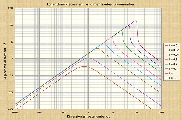
Primary Wave Attenuation Analysis, Fo < 2. Figure 2 depicts the variation of the logarithmic decrement δ1 for Fo < 2, as a function of σ*. The following conclusions are drawn: (1) The logarithmic decrement δ1 is maximum (in absolute value) at a value of σ* corresponding to the point of inflexion of the c*r versus σ* curve (Fig. 1). The value of σ* for which δ1 is a maximum (in absolute value) decreases with increasing Fo; and (2) the logarithmic decrement δ1 is minimized (in absolute value) at both ends of the σ* spectrum. As σ* → 0, δ1 → 0, corresponding to the kinematic wave case; as σ* → ∞, δ1 → 0, corresponding to the gravity wave case.
A general conclusion derived from Fig. 2 relates to the fact that for Fo < 2, primary waves will be subject to very strong attenuation in the dynamic band, and to very weak attenuation in the gravity and kinematic bands.
|
Fig. 2 Primary wave logarithmic decrement -δ1 versus dimensionless
wave
number σ*; curve parameter = Froude number Fo ( Fo < 2 ).
|
|
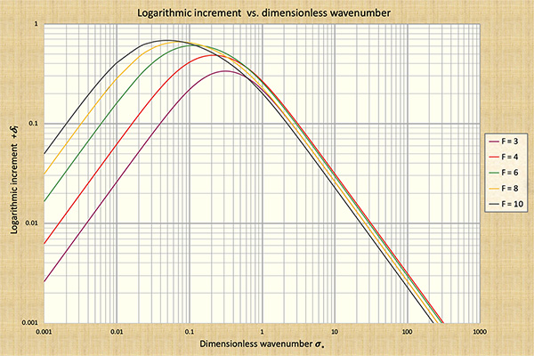
Primary Wave Amplification Analysis, Fo > 2. Figure 3 depicts the variation of the logarithmic decrement δ1, for Fo > 2, as a function of σ*. The following conclusions are drawn:
(1) The logarithmic decrement/increment δ1 has a maximum positive value at a value of σ* corresponding to the point of inflexion of the c*r versus σ* curve (Fig. 1). The value of σ* for which δ1 is a maximum decreases with increasing Fo; and (2) the logarithmic decrement δ1 is minimized at both ends of the σ* spectrum. As σ* → 0, δ1 → 0 corresponding to the kinematic wave case;
as σ* → ∞, δ1 → 0 corresponding to the gravity wave case.
A general conclusion derived from Fig. 3 relates to the fact that for Fo > 2, primary waves will be subject to very strong amplification in the dynamic band, and to very weak amplification in the gravity and kinematic bands.
|
Fig. 3 Primary wave logarithmic increment +δ1 , versus dimensionless wave
number σ*; curve parameter = Froude number Fo ( Fo > 2 ).
|
|
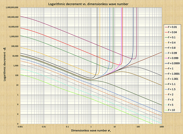
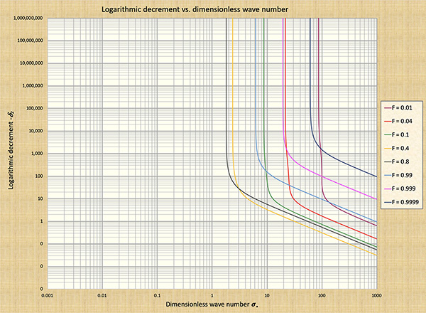
Secondary Wave Attenuation Analysis. Figures 4 (a) and 4 (b) depict the variation of the logarithmic decrement δ2 for 0.01 ≤ Fo 10 as a function of σ*. The following conclusions are drawn: (1) In subcritical flow, Fo < 1, the attenuation of the secondary wave is very strong, and the strength decreases as σ* increases in the gravity band (large σ*); (2) at critical flow, Fo = 1, the attenuation of the secondary wave is very strong, with a minimum around the center of the dynamic band (intermediate σ*); and (3) in supercritical flow, Fo > 1 the attenuation of the secondary wave has the pattern shown. For Fo ≥ 2, δ2 decreases as σ* increases.
|
(a)
|
(b)
Fig. 4 Secondary wave logarithmic decrement - δ2 versus dimensionless wave number σ*;
curve parameter = Froude number Fo : (a) 0.01 ≤ Fo ≤ 10; (b) 0.01 ≤ Fo ≤ 0.999.
|
|
11. DYNAMIC WAVE PROPAGATION
The propagation of a dynamic wave has been shown to be a function of two dimensionless parameters, the wave number σ* and the Froude number Fo. The wave number σ* can be interpreted as a ratio of two lengths Lo and L, in which L is the wavelength and Lo is the horizontal length in which the steady uniform flow drops a head equal to its depth. The square of the Froude number Fo is the ratio of twice the velocity head to the flow depth, where the velocity head huo is given by the following:
uo2
huo = ______
2 g
| (61) |
For Fo < 2, the celerity of a dynamic wave that propagates downstream is larger than the kinematic wave celerity, and smaller than the gravity wave celerity. In fact, the kinematic wave celerity constitutes a lower bound to which the dynamic value tends as the wave number σ* decreases. Conversely, the gravity wave celerity is an upper bound to the dynamic wave celerity as the
wave number σ* increases. To place this conclusion in the proper perspective, it is perhaps of interest to quote here from Stoker's work [(8), p. 486], regarding the celerities of small disturbances and progressive waves:
"What seems to happen is the following: small forerunners of a disturbance travel with the speed (gd)1/2 relative to the flowing stream, but the resistance forces act in such a way as to decrease the speed of the main portion of the disturbance far below the values given by (gd)1/2; i.e., to a value corresponding closely to the speed of a steady progressive wave that travels unchanged in form." |
In reviewing Stoker's work, it is apparent that his reference to a small disturbance is to a wave with a large σ* (gravity wave) and to progressive wave to that with a small σ* (kinematic wave). He proceeds to further elaborate on the limitations of methods of water routing based solely on the kinematic approach, for the cases in which the dynamic effects cannot be disregarded.
For Fo ≥ 2, the celerity of a dynamic wave that propagates downstream is smaller than the kinematic wave celerity and larger than the gravity wave celerity. In fact, the kinematic wave celerity is an upper bound to the dynamic value, whereas the gravity wave celerity is a lower bound to the dynamic value.
A significant conclusion regarding dynamic wave propagation can be obtained from the summary presented in Table 2. For primary waves, Fo = 2 is the threshold dividing the attenuation (Fo < 2) and amplification (Fo > 2) tendencies. For secondary waves, however, Fo = 1 is the threshold dividing the propagation upstream (Fo < 1) or downstream (Fo > 1) for gravity waves. Thus, Fo = 2 is verified to be as important a threshold value as Fo = 1 in describing the dynamics of open channel flow phenomena.
12. SUMMARY AND CONCLUSIONS
The propagation characteristics of various types of shallow water waves in open channel flow are calculated on the basis of linear stability theory. The celerity and attenuation functions of kinematic, diffusion, steady dynamic,
dynamic, and gravity waves are derived. For the most general case, i.e., the dynamic wave model, the propagation characteristics are expressed as a function of the steady uniform flow Froude number and the dimensionless wave number of the unsteady component of the motion.
For the dynamic model, the wave number spectrum is divided into three bands: (1) A gravity band corresponding to large wave number, in which the wave celerity is the gravity wave celerity; (2) a kinematic band corresponding
to a small wave number in which the wave celerity is the kinematic wave celerity; and (3) a dynamic band corresponding to midspectrum values of the wave number, in which the wave celerity falls between the gravity and kinematic
celerity values.
Primary dynamic waves propagate downstream, and they attenuate for Fo < 2 and amplify for Fo > 2. At the Fo = 2 threshold, primary dynamic waves neither attenuate nor amplify.
For Fo ≤ 1, secondary dynamic waves either propagate upstream or downstream, depending on the wave number. At Fo = 1, secondary dynamic waves remain stationary or propagate downstream, depending on the wave number. For Fo > 1, secondary waves propagate downstream. Secondary waves attenuate throughout the entire wave number spectrum.
13. APPLICATIONS
The analysis of the foregoing sections provides an appropriate framework for the systematic study of shallow water waves in open channel flow. Numerous applications are envisioned, among which some of the most important are:
The assessment of the accuracy of kinematic and diffusion wave models, and the determination of the criteria for their applicability.
The study of the formation of roll waves in open channel flow. The present theory validates the observed fact that roll waves are formed for Fo > 2, since there can be no wave amplification for Fo ≤ 2 (using Chezy friction).
The theory enables a comparison of the various approximate wave models and an assessment of their capabilities and limitations.
Lastly, the theory provides a coherent treatment of the subject of wave propagation in open channel flow. The conclusions may prove of interest to engineers dealing with unsteady open channel flow phenomena.
APPENDIX I. REFERENCES
-
DeSaint-Venant, B. 1871. "Theorie du Mouvement Non-permanent des Eaux avec Application aux Crues des Rivieris et I' Introduction des Varies dans leur Lit," Competes Rendus Hebdomadaires des Seances de l'Academie des Science, Paris, France, Vol. 73, 148-154.
-
Henderson, F. M. Open Channel Flow. 1966. The MacMillan Co., New York, N.Y.
-
Lagrange, I. L. 1869. "Mémoire sur la Théorie du Mouvement des Fluides," Bulletin de la Classe des Sciences Academie Royal de Belique, No. 1783, pp. 151-198.
-
Liggett, J. A. 1975. "Basic Equations of Unsteady Flow," Unsteady Flow in Open Channels, K. Mahmood and V. Yevjevich, ed., Vol. 1, Water Resources Publications, Fort Collins, Colo.
-
Lighthill, M. J., and G. B. Whitham. 1955. "On Kinematic Waves I, Flood Movement in Long Rivers," Proceedings of the Royal Society of London, Vol. A229, May, 281-316.
-
Lin, C. C. 1966. The Theory of Hydrodynamic Stability, 1st ed., The Cambridge University Press, London, England.
-
Ponce, V. M., and K. Mahmood. 1976. "Meandering Thalwegs in Straight Alluvial Channels," Proceedings of the 3rd Annual Symposium, ASCE, Waterways, Harbors, and Coastal Engineering Division, Vol. 2, Aug., 1418-1441.
-
Stoker, J. J. 1957.Water Waves, the Mathematical Theory with Applications, Wiley Interscience Publishers, Inc., New York, N.Y.
-
Woolhiser, D. A., and J. A. Liggett. 1967. "Unsteady One-Dimensional Flow over a Plane-The Rising Hydrograph," Water Resources Research, Vol. 3, No. 3, Third Quarter, pp. 753-771.
-
Wylie, C. R. 1966. Advanced Engineering Mathematics, 3rd ed., McGraw-Hill Book Co., New York, N.Y.
APPENDIX II. NOTATION
The following symbols are used in this paper:
A = parameter, defined by Eq. 39;
a = integer;
B = parameter, defined by Eq. 40;
C = parameter, defined by Eq. 41;
Cf = Chezy coefficient;
D = parameter, defined by Eq. 50;
d = depth of flow;
E = parameter, defined by Eq. 51;
Fo = Froude number of steady uniform flow;
f = friction factor, defined by Eq. 7;
g = acceleration of gravity;
hu = velocity head;
k = integer;
L = wavelength;
Lo = length in which the steady uniform flow drops a head equal to its
depth;
l = integer;
p = integer;
Sf = friction slope;
So = bed slope;
T = wave period;
u = mean velocity;
β*I = amplitude propagation factor;
β*R = dimensionless frequency;
γ = unit weight of water;
δ = logarithmic decrement;
ζ = a type of kinematic flow number, as defined by Eq. 37;
θ = parameter, defined by Eq. 43;
σ* = dimensionless wave number;
τ = bottom shear stress; and
∞ = infinity.
Subscripts
d = diffusive wave;
g = gravity wave;
I = imaginary;
k = kinematic wave;
o = steady uniform flow;
R = real;
r = relative to the main flow;
s = steady dynamic wave;
1 = primary dynamic wave; and
2 = secondary dynamic wave.
Superscripts
' = perturbed variable; and
* = dimensionless function.
|
|
|