1. INTRODUCTION
The dichotomy between kinematic and dynamic waves and its relation to scale has
defied complete understanding in the past.
The matter has been
elucidated by Ponce and Simons (1977), who identified the appropriate
dimensionless wavenumber and
plotted dimensionless relative wave celerities across
the spectrum of dimensionless wavenumbers. In addition, they
clarified the propagation characteristics of various types
of shallow water waves, including their celerity and attenuation properties.
Herein, we review the Ponce and Simons theory
and explain its significance. The aim is to showcase
the importance of wave propagation in hydraulic engineering modeling practice.
2. THE THEORY EXPLAINED
Shallow wave propagation in open-channel flow is governed by the equations of water continuity and motion,
generally referred to as the Saint Venant equations (Ponce, 2014). These are a set of two partial differential
equations for which there is no complete analytical solution. This theoretical difficulty was circumvented
by Ponce and Simons (1977), who
linearized the governing equations and applied the tools of linear stability
to formulate a characteristic algebraic equation which retained the essence of the solution.
The proper definition of dimensionless wavenumber allowed the
calculation of celerity and attenuation functions across the entire spatial domain.
The results described wave propagation for several types of shallow waves,
throwing much needed light on the wave phenomena.
3. FORCES AND WAVE TYPES
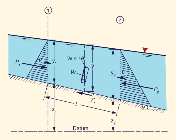
There are four forces in the analysis of unsteady open-channel flow
(Fig. 1):
The following types of shallow water waves are in general use: (1) kinematic, (1a) diffusion, (2) mixed kinematic-dynamic, and (3) dynamic. Kinematic waves are governed solely by gravity and friction (Fig. 2); diffusion waves by gravity, friction and the pressure gradient; mixed kinematic-dynamic waves by all four forces, namely gravity, friction, the pressure gradient, and inertia (Fig. 3); and dynamic waves solely by the pressure gradient and inertia (Table 1).
At the outset, it is necessary to point out that there exists currently a semantic confusion regarding
what to call the different types of waves. What we call here mixed kinematic-dynamic waves
have been generally referred
to in the literature
as "dynamic," following the work of Fread (1973). On the other hand,
the classical dynamic waves, i.e., the dynamic waves of
Lagrange (1788), have been often referred to as "gravity" waves.
In this work, we follow the naming indicated in Column 2 of
The term "kinematic wave" was introduced by Lighthill and Whitham in their seminal paper, purportedly to contrast the then well established dynamic waves, which transport energy, to waves that transport mass. We quote here directly from Lighthill and Whitham (1955):
Classical dynamic waves transport only energy; therefore, it follows that mixed kinematic-dynamic waves transport both mass and energy. In the resolution of this dichotomy may lie the strong attenuating (dissipating) tendency of mixed kinematic-dynamic waves.
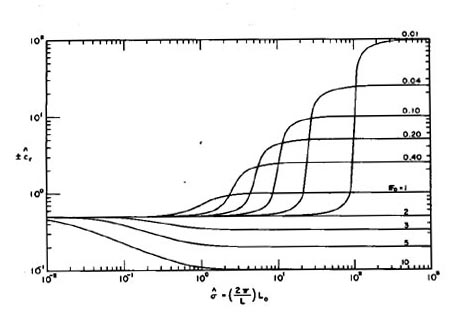
4. PONCE AND SIMONS' FINDINGS Ponce and Simons plotted dimensionless relative wave celerities across the spectrum of dimensionless wavenumbers and specialized their findings into each one of the four wave types described in Table 1. Crucial to this effort was the identification of the dimensionless wavenumber σ* :
in which Lo = characteristic reach length, the length of channel in which the steady uniform flow drops a head equal to its depth (Lighthill and Whitham, 1955):
in which do = steady uniform flow depth, and So = channel bed slope. Figure 4 shows dimensionless relative wave celerities across the dimensionless wavenumber spectrum. Given c = wave celerity, the relative wave celerity cr is:
in which u o = steady uniform flow velocity. The dimensionless relative wave celerity cr* is:
The range of dimensionless wavenumbers shown in Fig. 4 spans six orders of magnitude, encompassing from the longest waves (kinematic, of small σ*), to the shortest waves (dynamic, of large σ*). Herein, we refer to Fig. 4 as the S-curve. All four wave types (kinematic, diffusion, mixed kinematic-dynamic, and dynamic) are contained in the S-curve.
5. KINEMATIC WAVES
Kinematic waves are governed solely by gravity and friction. Their celerity is constant and
equal to the kinematic wave celerity, or
Seddon celerity, and they do not attenuate (with some exceptions
for nonlinear waves).
in which T = channel top width, Q = discharge, and y = flow depth. The Seddon, or kinematic wave celerity, is alternatively expressed as follows (Ponce, 2014):
in which β = exponent of the discharge-flow area rating:
The relative kinematic wave celerity, or kinematic wave celerity relative to the flow velocity, is:
The dimensionless relative kinematic wave celerity is:
The value of β is a function of channel friction and cross-sectional shape. For Chezy friction in a hydraulically wide channel: β = 1.5. In this case:
For Froude numbers in the stable regime, F ≤ 2,
which corresponds to Vedernikov numbers V ≤ 1 (Ponce, 1991),
In the Ponce and Simons theory, wave attenuation is a function of the change in relative dimensionless wave celerity with change in dimensionless wave number. In other words, attenuation is caused by the change in celerity with wave size. For the case of (dcr* /dσ*) = 0, there can be no wave attenuation; therefore, kinematic waves do not attenuate.
The above conclusion,
while strong, is strictly valid only for the linear theory
in hydraulically wide channels. In the general nonlinear case,
kinematic waves may undergo changes in shape, either steepening or flattening, depending on the
cross-sectional shape (Ponce and Windingland, 1985).
In summary, kinematic waves travel with the Seddon celerity and, in general, they are not subject to attenuation. The condition of a wave being kinematic depends on the dimensionless wavenumber, with the wave becoming more kinematic as σ* decreases (See Fig. 4 for the appropriate values).
The criterion for the applicability of
a kinematic wave in open-channel flow
has been developed by Ponce et al. (1978).
in which T = wave period; So = bed slope; uo = mean velocity; and do = mean flow depth.
6. DIFFUSION WAVES
Diffusion waves are governed by gravity, friction, and the pressure gradient.
The inclusion of the pressure gradient in the formulation of a diffusion wave
provides diffusion, i.e., the wave is capable of undergoing attenuation, or
dissipation; therein its name, diffusion wave. The origin of the name
may be traced back to the work of Lighthill and Whitham (1955), who
reckoned that diffusion could be added to a kinematic wave by
including the pressure-gradient term in the formulation.
In Ponce and Simons' theory, the celerity of a diffusion wave is, as an approximation,
the same as that of the neighboring kinematic wave (in the dimensionless
wavenumber spectrum). The difference is in the attenuation function.
Unlike the kinematic wave, for which the attenuation is zero,
the diffusion wave is subject to a small but finite amount of attenuation. The attenuation
is a function of the dimensionless wavenumber
σ* , and, as expected,
increases with it.
To characterize the magnitude of the wave attenuation, Ponce and Simons used the logarithmic decrement δ,
which measures the attenuation after one (sinusoidal) propagation period. For the diffusion wave, the logarithmic decrement is:
which reduces to δd ⇒ 0 as σ* ⇒ 0, thus coalescing into a kinematic wave.
A diffusion wave has a wider range of applicability than a kinematic wave. In cases where
a kinematic wave fails, a diffusion wave may be applicable. The criterion for the applicability of
a diffusion wave has been developed by Ponce et al. (1978).
The criterion is based on the following
dimensionless inequality:
in which g = gravitational acceleration.
In Figure 4, diffusion waves would fall to the right of kinematic
waves, in the middle of the dimensionless wavenumber range,
0.1 ≤ σ* ≤ 10, depending on the Froude number. The lower the
prevailing Froude number in the stable range (F ≤ 2), the greater
the range of applicability of diffusion waves.
7. MIXED KINEMATIC-DYNAMIC WAVES
Mixed kinematic-dynamic waves are governed by all four forces: gravity, friction, pressure gradient, and inertia. As such, a mixed kinematic-dynamic
wave represents the most complete formulation of shallow-water waves
in open-channel flow; however, it is not without its pitfalls.
Under typical subcritical flow conditions, mixed kinematic-dynamic waves are
subject to
very strong attenuation, to the extent that often their existence
may be placed under question. This fact was recognized by Lighthill and Whitham (1955) when they stated:
"Under the conditions appropriate for flood waves... the dynamic (sic) waves
rapidly become negligible, and it is the kinematic waves,
following at a slower speed, which assume the dominant role."
Thus, the mixed kinematic-dynamic waves,
lying directly on the rising limb of the S-curve (Fig. 4), are generally subject to
very strong attenuation. The rate of attenuation increases with the
rise on the curve, achieving a peak at the point of inflection.
These propositions were demonstrated by Ponce and Simons (1977) in their
analysis of the mixed kinematic-dynamic wave model. The results are
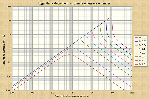
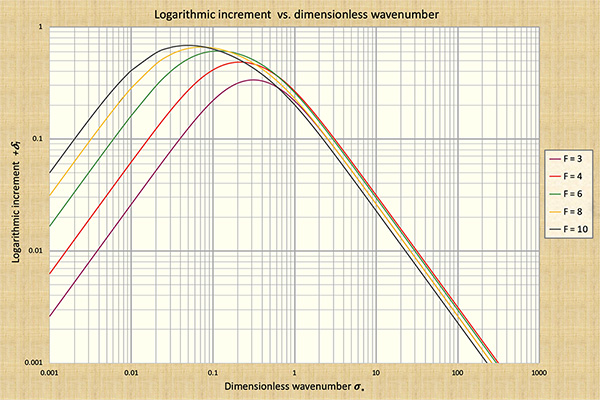
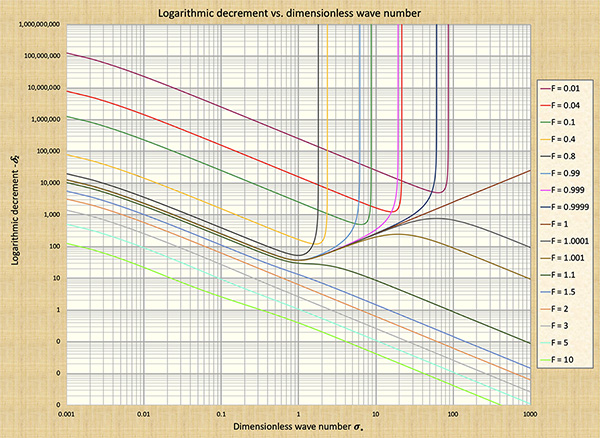
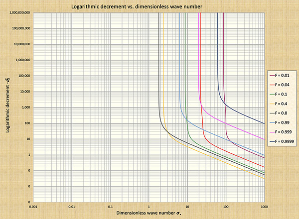
summarized in Figs. 4, 6, 7, and 8.
The following conclusiones are drawn from Fig. 4:
The following conclusiones are drawn from Fig. 6:
The following conclusiones are drawn from Fig. 7:
The following conclusiones are drawn from Fig. 8:
In summary, the findings of Ponce and Simons (1977) serve to clarify the relation between kinematic and mixed kinematic-dynamic waves: While the former do not attenuate, the latter are subject to very strong attenuation, particularly in the subcritical regime, where it matters most. Kinematic waves are applicable to overland flow and flood routing; mixed kinematic-dynamic waves are primarily applicable to dam-breach flood waves and, in unusual cases, to flood routing. Diffusion waves, lying in between kinematic and mixed kinematic-dynamic waves, have small amounts of diffusion and are, therefore, able to properly simulate flood waves.
8. DYNAMIC WAVES
The dynamic waves of classical mechanics are governed solely by the pressure gradient
and inertia. They lie to the right of the dimensionless wavenumber spectrum,
corresponding to the top of the S-curve of Fig. 4.
For the most part, their celerity is constant and equal to the dynamic wave celerity, or
classical Lagrange celerity, expressed as follows:
This equation reveals the two components of dynamic wave propagation.
The
relative dynamic wave celerity
is:
The dimensionless relative dynamic wave celerity is:
which is recognized as the reciprocal of the Froude number:
Equation 17 is represented in Fig. 4. For instance, for F = 0.1 (pink curve), the value of
dimensionless
relative wave celerity approaches 10 to the right of the scale.
The following conclusiones regarding dynamic waves are drawn from Fig. 4:
9. SUMMARY
The theory of shallow wave propagation of Ponce and Simons (1977)
is reviewed and clarified, with aim to
showcase its importance in understanding the mechanics of unsteady open-channel flow.
REFERENCES
Fread, D. L. 1973. Technique for implicit dynamic routing in rivers with tributaries. Water Resources Research,
9(4), 338-351.
Lagrange, J. L. 1788. Mécanique analytique, Paris, part 2, section II, article 2, p. 192.
Lighthill, M. J., and G. B. Whitham. 1955.
On kinematic waves: I. Flood movement in long rivers. Proceedings, Royal Society of London, Series A, 229, 281-316.
Ponce, V, M., and D. B. Simons. 1977. Shallow wave propagation in open-channel flow. Journal of the Hydraulics Division, ASCE, Vol. 103, No. HY12, December, 1461-1476.
Ponce, V, M., R. M. Li, and D. B. Simons. 1978.
Applicability of kinematic and diffusion models. Journal of the Hydraulics Division, ASCE, Vol. 104, No. HY3, March, 353-360.
Ponce, V. M., and D. Windingland. 1985. Kinematic shock: Sensitivity analysis,
Journal of Hydraulic Engineering, ASCE, 114(4), 600-611.
Ponce, V. M. 1991. New perspective on the Vedernikov number. Water Resources Research, Vol. 27, No. 7, 1777-1779, July.
Ponce, V. M. 2014.
Engineering hydrology: Principles and practices. Second edition, online textbook.
Ponce, V. M. 2014.
Fundamentals of Open-channel Hydraulics. Online textbook.
Ponce, V. M. and B. Choque Guzmán. 2019.
The control of roll waves in channelized rivers. Link No. 36023
in ponce.sdsu.edu.
Seddon, J. A. 1900. River hydraulics.
Transactions, ASCE,
Vol. XLIII, 179-243, June.
| |||||||||||||||||||||||||||||||||||||||||||||||||||||||||||||||||||||||||||||||||||||||||||||||||||||||||||||||||||||||||||||||||||||||||||||||||||||||||||||||||||||||||||||||||||||||||||||||||


| 220513 |