|
|
|
| Contents | References | ||
| 1. Introduction
2. Geology 3. Geomorphology |
4. Climatology
5. Hydrology 6. Ecology |
7. Ecohydrology
8. Hydroclimatology 9. Bioclimatology |
10. Ecohydroclimatology
11. Case Studies 12. Summary |
1. INTRODUCTION
|
|
In Nature, everything is related. The Earth's crust and its environment, including climate, water, soils, nutrients, flora and fauna interact with each other in time and space in endless and demonstrably self-perpetuating ways. In the meantime, humans have endeavored to explore Nature by dividing it into convenient fields. This approach has given way to several natural sciences, among them, geology, geomorphology, climatology, hydrology, and ecology. Over the past two centuries, the development of scientific fields has produced a wealth of knowledge; this knowledge has been forthcoming, but it has been at the expense of the holistic view.
Over the past three decades, a new horizon is in place. It is no longer sufficient to concentrate on one science. Such an approach may achieve disciplinary wonders, but it fails to describe the interaction between two closely related fields, for instance, hydrology and ecology. The new paradigm is the interdisciplinary approach, which strives to connect related fields into a knowledge continuum seeking to describe Nature in a more comprehensive, holistic way. Thus, the rise of the fields of ecohydrology and hydroclimatology.
Ecohydrology studies the relations between flora/fauna and the hydrologic processes embodied in the water cycle. Plants and animals cannot exist without water; thus, the rationale for the study of the relations between them. These relations are at the crux of the relatively new science of ecohydrology.
Climate and the hydrologic cycle interact with each other in a myriad of ways. Simply stated, one could not be described without the other. A case in point: Does rain produce vegetation? Or, does vegetation produce rain? This dichotomy is at the center of the science of hydroclimatology, the study of the relations between climate and water, including rivers, lakes, groundwater, and oceans.
A step in the right direction is the new science of ecohydroclimatology, which is, by definition, a combination of ecohydrology and hydroclimatology. Flora and fauna interact with the surrounding geology, water, and climate in a variety of ways, too many and too complex to be aptly described with a disciplinary perspective. The fundamental aim of Nature is stability, embodied in the concept of dynamic equilibrium, which recognizes the presence of change within an essentially stable system. Then, ecohydroclimatology is the study of the relations between ecology, hydrology, and climatology, aimed at clarifying the natural laws that underpin dynamic equilibrum.
This report explores concepts of geology, geomorphology, climatology, hydrology, and ecology, with the objective of contributing to the development of a seamless, interdisciplinary approach. The aim is to research the "whys" of Nature currently hiding at or near the limits between these disciplines. Relevant questions are likely to be answered under the new optics of ecohydroclimatology. It is argued herein that geomorphology serves as the "glue" that ties the other fields together. Several practical examples help make the case for geomorphology a veritable one.
2. GEOLOGY
|
|
Geology is the study of the Earth's crust, the rocks from which it is composed, and the processes by which they undergo change. Geology can be used as the means to study the history of the Earth, its past climates, and the evolutionary history of life. Closely related to geology is the field of geography, which describes the Earth and all of its natural and human complexities. Geography describes the oceans, land, mountains, valleys, rivers, lakes, and other distinguishable features of the Earth's surface.
The domain of geology is the Earth's crust, loosely interpreted as the layer on the surface about
Geology studies the various types of rocks on the Earth's surface, including igneous, sedimentary, and metamorphic, and the information that can be weaned from geologic history for the benefit of humankind. Geology interacts with the climate and fundamental laws of physics and chemistry to produce an Earth that, while smooth and round when observed from space, nevertheless may appear rough or irregular when viewed at close range.
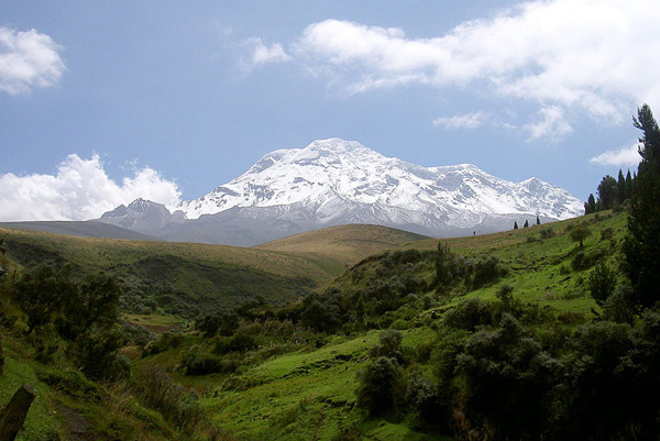
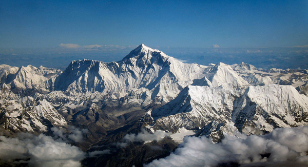
A simple calculation will serve to illustrate the dichotomy. The highest point on the Earth's surface
is the peak of Mount Everest, which straddles the countries of Nepal and China, at an altitude of
|
8,848 × 0.001 κ = _________________ = 0.000883 0.25 × 40,075 | (1) |
Yet anybody that has climbed Mount Everest will attest to the challenge (Fig. 1). Tectonic uplift, to which Mount Everest owes its demonstrable prowess, is thus, new, from a geologic standpoint.
|
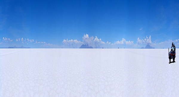
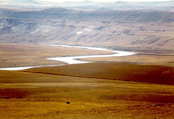
On the other extreme, there are portions of the Earth's surface that are extremely flat; for instance, the Uyuni Salt Flat, in southwest Bolivia, the world's largest, encompassing 10,582 km2 of surface area. The salt lake, covered with a few meters of salt crust, is of extraordinary flatness, featuring altitude variations of less than one meter over the entire area of the lake (Fig. 2).
Geographically, Uyuni lies at the terminus of the large endorheic Altiplano Basin of Peru and Bolivia, collecting the salt which originates in the basin of Lake Titicaca and those of other lakes in the region. Uyuni's flatness conveys a message of extensive subsidence and sedimentation, and, geologically speaking, of time gone by. The source of all salt is rock weathering. Yet the fate of salt is double-pronged: In exorheic basins, it winds up in the ocean; in endorheic basins, it collect in salt lakes and, in extreme cases, in salt flats like Uyuni.
|
Geology by itself does not explain all processes on the surface of the Earth. Other factors include atmospheric and oceanic circulation, tectonism, volcanic activity, continental location, latitude, and, given the relative smoothness of the Earth, the form of the surface. All of these factors have a role in determining the character of the processes.
Geology is only the first of a chain of related processes that condition and make possible life on Earth. Geomorphology may well be the second.
3. GEOMORPHOLOGY
|
|
Geomorphology is the scientific study of landforms and the processes that shape them. The aim is to understand why landscapes look the way they do, to study landform history and evolution, and to predict changes through field observation and modeling.
Geomorphology is affected by processes of tectonic uplift and subsidence, erosion and deposition, and the action of natural agents such as gravity, water, wind, ice, and fire. Geomorphology is also affected by living things, such as plants, animals, and human beings.
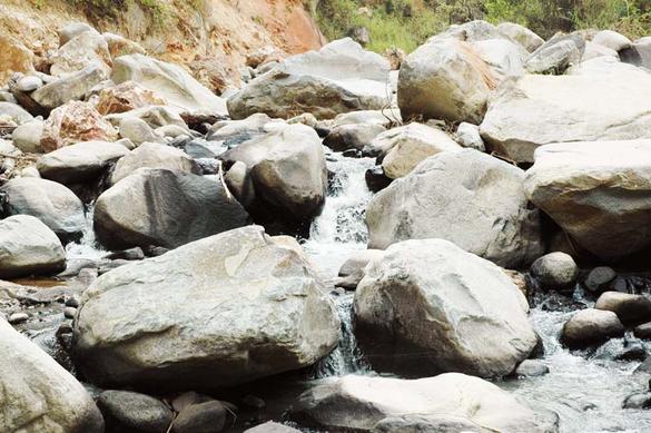
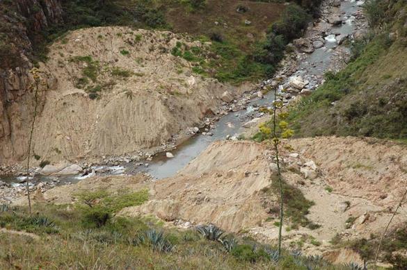
The dual processes of uplift and subsidence, and erosion and deposition are fundamentals tenets of geomorphology. Through uplift the Earth's crust goes up, and through subsidence it comes down. Erosion in the highlands and deposition in the lowlands contribute to shape the form of the landscape. Physical, chemical, and biological processes combine to break and disaggregate the rocks. Gravity, rainfall, and runoff are responsible for the dislodgement, entrainment, and transport of rock fragments and soil particles (Fig. 3).
|
The shape of the Earth's hydrologic basins, typically concave when observed from above, acts to make sure that not all particles dislodged make it all the way to the ocean. A sizable fraction of the eroded material always stays behind to form the alluvial valleys. The more extensive and deeper the valleys, presumably the older they are.
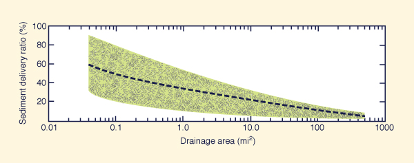
This fact of Nature is admirably expressed in the concept of sediment yield (Ponce, 1989). The amount of sediment delivered to a downstream point (i.e., the sediment yield) is always a fraction of the amount of sediment produced in the uplands. Predictably, the sediment delivery ratio decreases with an increase in the size of the basin, as shown schematically in Fig. 4.
|
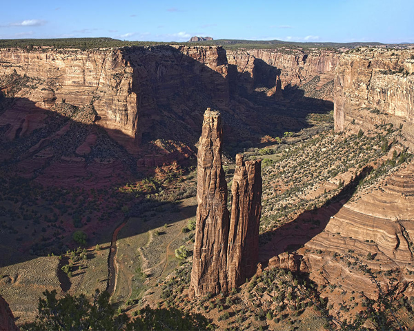
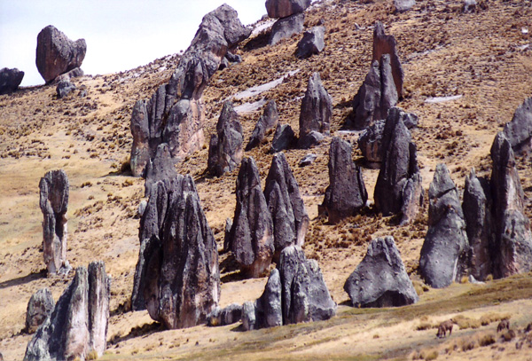
The science of geomorphology is divided into several subfields: (1) terrestrial, (2) fluvial, (3) lacustrine, and (4) ocean. Actually, the patterns and shape of the Earth's surface are infinite; there appear to be no general rules or laws to follow; see, for instance, the natural rock sculptures shown in Figs. 5 and 6. Thus, when geomorphological knowledge is required to support concerted action and/or management, there is no substitute for observation and experience.
|
|
Geomorphology interacts with hydrology in a myriad of ways; in turn, hydrology interacts with geology, ecology and climate. The relations are complex and it is difficult to discern cause-effect relations. The best that can be stated in this regard is that all these fields are intrinsically connected and thoroughly intertwined. Yet geomorphology stands out as the unifying mechanism appearing to oblige its sister sciences.
Exorheic vs endorheic drainages
The most significant interaction between geomorphology and hydrology is provided by runoff, which begins shortly after precipitation hits the ground. After hydrologic abstractions, runoff on the Earth's surface collects as drainage into streams and rivers. Drainage can be of two types: (1) exorheic, and (2) endorheic. Exorheic drainages return water to the ocean, closing the hydrologic cycle. On the other hand, endorheic drainages do not reach the ocean, returning instead to the atmosphere, short-circuiting the cycle.
Peripheral continental regions are almost always exorheic, with streams and rivers discharging into the nearest ocean. In contrast, non-peripheral continental regions could be endorheic, with streams and rivers discharging into closed basins, collecting into inland lakes.
Two factors help determine whether a drainage system at a given location will be either exorheic or endorheic: (1) the size of the continent, and (2) the general shape of the land, as modified by (a) uplift and subsidence, and (b) erosion and deposition. The larger the continent, the greater the chance that it will have some endorheic continental regions.
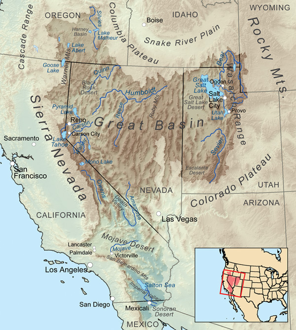
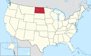
The United States is a good example of a large subcontinent featuring both exorheic and endorheic drainages. The basins of the Mississippi, Columbia, and Colorado rivers are exorheic, to focus only on the three largest basins. Yet the Great Basin, which comprises most of Nevada and parts of California, Oregon and Utah, is endorheic (Fig. 7).
|
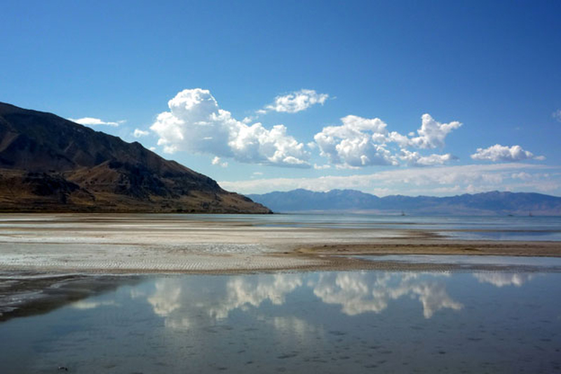
Endorheic basins are of two types: (1) fully endorheic, or closed, basins, and (2) partially endorheic, or open, basins. Fully endorheic basins have no outlet to the ocean; in contrast, partially endorheic basins experience some drainage, either permanently, seasonally, or pluriannually. For instance, the basin of the Great Salt Lake of Utah is fully endorheic. As a result, the Great Salt Lake is an hypersaline lake, its salinity varying from 50 to 270 ppt (parts per thousand), depending on location and lake level. By comparison, the salinity of the open oceans is about 35 ppt.
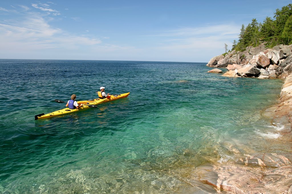
In contrast to the Great Salt Lake, the Great Lakes of North America
are partially endorheic.
The Great Lakes drain into the Atlantic Ocean
through the Saint Lawrence river and, therefore, feature fresh water.
In fact, the water of Lake Superior, the most upstream
of the Great Lakes, is among the freshest in the Earth, with a
salinity of 0.063 ppt. [By comparison,
the salinity of typical fresh waters is around 0.2 to
|
In geologic time, closed basins continue to collect and accumulate salt,
while open basins feature fresh water of varying salinity, typically between 0.5 to 10 ppt, depending
on the degree of endorheism. A greater degree of endorheism leads to waters of higher salinity.
For instance, Lake Titicaca, which straddles Peru and Bolivia, in South America,
flushes about 2%
of its volume on an annual basis and, therefore,
features a relatively low salinity content of about 1 ppt (Fig. 9).
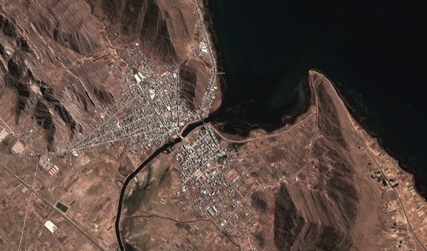
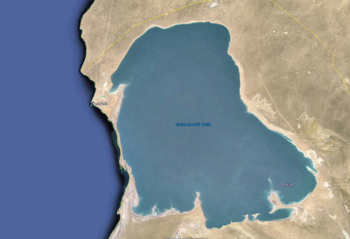
In contrast, the Caspian Sea, in eastern Europe and Asia,
a partially endorheic system, has a salinity content of
|
|
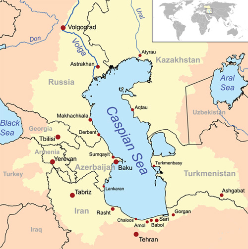
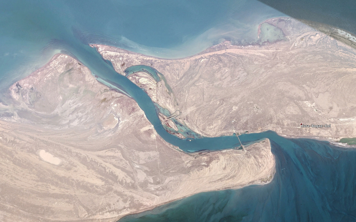
Significantly, the Caspian Sea drains into Garabogazkol Basin, the terminus of its closed drainage. The latter basin features a salinity of 345 ppt, which is about 10 times that of the open ocean. The channel entrance is about 200 m wide (Fig. 11).
|
It is seen that geomorphology determines hydrology and drainage, and that drainage determines salinity. In turn, salinity determines ecology, giving rise to the possibility of different kinds of living organisms. Thus, the link between geomorphology and ecology is demonstrated.
4. CLIMATOLOGY
|
|
Climatology is the study of climate, i.e., of weather conditions in a certain region, averaged over a period of time. Weather and climate depend on the spatial scale of interest, which varies widely, from global to mesoscale, regional, local, micro, and even nanoscale. The prediction of weather is difficult at best, due to the many relations between and within the spatial scales. However, climate, being an average of the weather, is somewhat more predictable.
Climatic factors
Several factors affect climate. The primary factors are: (1) latitude, (2) altitude, (3) precipitation, (4) temperature, (5) relative humidity, and (6) season. Secondary factors include: (1) atmospheric currents, (2) ocean currents, (3) continental location, (4) orographic barriers, (5) volcanic eruptions, (6) wildland fires, (7) land-surface condition, and recently, (8) anthropogenic climate change.
Weather and climate are energy-driven, and the source of all energy is the Sun. Latitude is the fundamental parameter; proximity to the Sun determines temperature, which conditions the climate. Temperatures are highest along the equator and lowest at the poles. Rotation of the Earth on its axis assures diurnal/nocturnal variations. Rotation of the Earth around the Sun assures annual (seasonal) variations.
Depending on latitude, the climate can be either: (a) tropical, (b) subtropical, (c) temperate, (d) boreal/austral, (e) subpolar, or (f) polar. Tropical climates have the highest temperatures, while polar climates have the lowest. Proximity to the Sun is the determinant factor in near-ground air temperature. Biological activity thrives at high temperatures; thus, tropical regions have the highest rates of biological activity, through plant photosynthesis and animal respiration.
The Earth is a spheroid at a distance of 149,600,000 km from the Sun. The points closest to the Sun are located along the equator. The peak of the Chimborazo volcano, in Ecuador, at an altitude of 6,268 m, is the point on Earth which is closest to the Sun (Fig. 12).
|
All factors determining climate are related. Latitude and altitude determine temperature. Precipitation determines the type and density of vegetation; therefore, it affects the temperature and, correspondingly, the climate. The lowest temperature ranges correspond to humid rainforests, while the highest are typical of superarid deserts. Relative humidity is also very much related to climate; it is low in superarid deserts and high in humid rainforests.
Atmospheric and ocean currents are responsible for mesoscale effects such as the El Niño Southern Oscillation (ENSO). ENSO refers to an event described by a band of sea-surface temperatures which are abnormally warm (El Niño) or cold (La Niña) for long periods of time, and which develop along the tropical western coast of South America, causing marked climatic changes along the tropics and the subtropics. Typical El Niño effects are extreme floods and droughts, which generally lead to loss of life and property damage.
Continental location (relative to the nearest ocean) affects climate because the combined global continental land surface represents only about 30% of the world's surface area. Thus, it can be surmised that about two-thirds of the global weather is effectively controlled by ocean processes. Due to the high specific heat of water, surface temperature gradients are much smaller over the oceans than over land. Therefore, peripheral continental regions are subject to less temperature variability that inland continental regions. This fact give rise to three definite climate types: (1) hyperoceanic, subject to strong ocean control, (2) oceanic, with mild ocean control, and (2) continental, with very little, if any, ocean control (Fig. 13) (Pulgar et al., 2010).
|
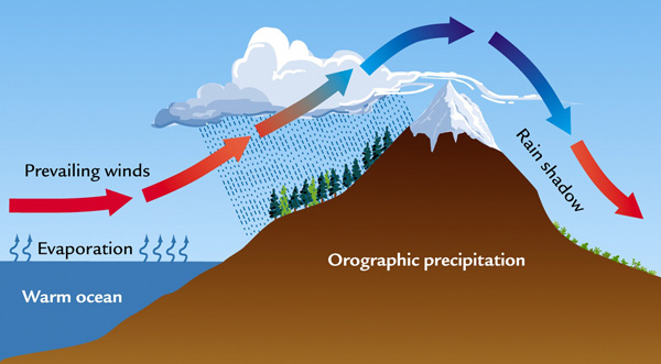
Orographic barriers affect the climate by influencing the spatial distribution of precipitation. On the windward side of a mountain, air mass lifting due to the presence of the physical barrier usually provides enough cooling to produce precipitation. On the leeward side (rain shadow), the same air mass is forced to descend, warming up and inhibiting precipitation (Fig. 14).
|
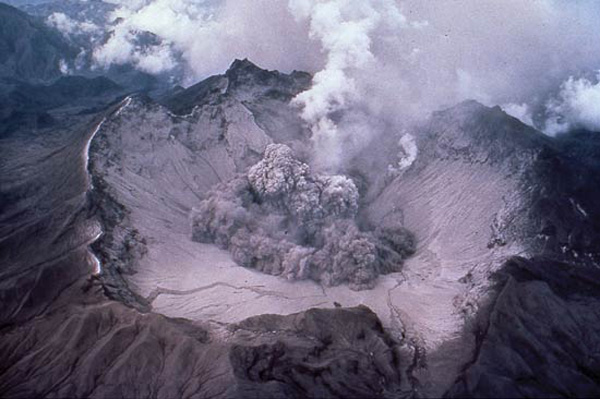
Volcanic eruptions change the precipitation patterns by increasing the concentration of particulates in the air, which promotes coalescence, resulting in increased precipitation. Depending on the size of the eruption and the amount of particulates (ash) released, the effects could be regional, and sometimes even global. That was the case of the 1993 eruption of Mount Pinatubo, in the Phillipines (Fig. 15), the second largest terrestrial eruption since Krakatoa in 1883. The eruption of Mount Pinatubo caused global temperatures to drop by about 0.5°C in the following two years (1991-93).
|
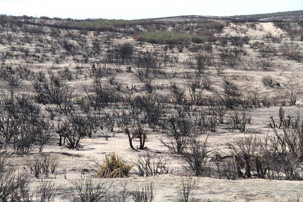
Wildland fires, both natural and human induced, affect the climate in very much the same way as volcanic eruptions, albeit to a lesser degree and geographical extent. Typically, wildfires lead to increased local/regional precipitation, increased erosion of the soil mantle and deposition elsewhere, and changes in weather and possibly even climate, although the latter effects are likely to be temporary, lasting only until full recovery of the native vegetation.
Figure 16 shows the aftermath of the Shockey fire, in Tierra del Sol, San Diego County, California. The fire, which started on September 23, 2012, lasted several days and burned 2,553 acres of chaparral vegetation. Thirty structures were destroyed and one life was lost.
|
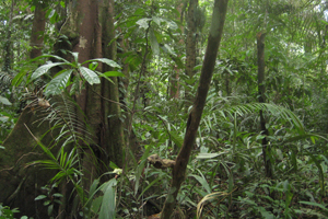
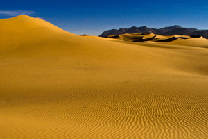
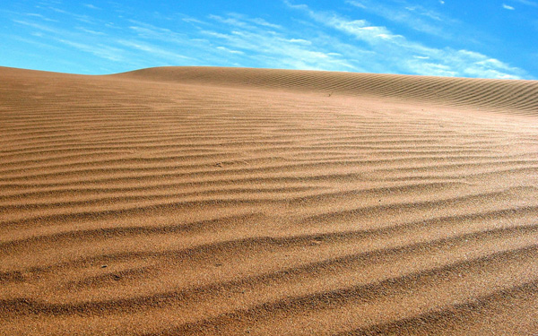
Land-surface topography and condition also affect weather and climate, although their effects are not readily discernible. The fundamental physical parameter is the albedo, the coefficient of reflectivity of the Earth's surface toward short-wave radiation. While the albedo of a rainforest varies in the range 0.07-0.15, that of a superarid desert is in the range 0.30-0.60 (Fig. 17).
|
Changes in albedo, whether natural or anthropogenically induced, are likely to alter the near-surface radiation balance and lead to changes in precipitation patterns (Ponce et al., 1999). Anthropogenic increases in albedo produce a condition referred to as desertification; conversely, anthropogenic decreases in albedo lead to humidification. Desertification is a problem in ecosystems around the world that are subject to anthropogenic pressure, such as deforestation, overcultivation, or overgrazing.
Anthropogenic climate change is the newest factor in climatology. After nearly 25 years of study, mainstream science has concluded that the concerted burning of fossil fuels (to drive industrial development and vehicular transportation) has produced an imbalance between photosynthesis and respiration at the global scale (http://www.ipcc.ch; Ponce, 2011). This imbalance has lead to an increase in atmospheric carbon dioxide, from about 290 ppm at the beginning of the 20th century, to 400 ppm at the present time (July 2015) to heed the most currently available data. By retaining heat through vibration, the diatomic molecule of carbon dioxide (CO2) produces a greenhouse effect, which results in increased near-surface air temperatures (Arrhenius, 1896) (Fig. 18).
|

Continuing its inexorable rise, the excess atmospheric carbon dioxide is causing marked climatic changes, such as increased average surface temperatures, increased icecap and glacier melt, rise in mean ocean levels, and stronger extremes in weather, such as floods, droughts, hurricanes, and tsunamis.
Classification of climate
The fundamental parameters in climate classification are average temperature and mean annual precipitation. In tropical and subtropical regions, temperature varies with elevation, while precipitation varies primarily with continental location and the presence/absence of orographic features. A simple climatic classification based only on precipitation may be advanced for the tropics and the subtropics.
The basis of the climatic classification is the mean annual global
terrestrial precipitation Pagt.
Table 1 shows the conceptual climatic classification. Line 1 shows the
classification in terms of mean annual precipitation Pma (mm), into eight (8) humidity provinces: superarid (Pma ≤ 100),
hyperarid (100 < Pma ≤ 200),
arid (200 < Pma ≤ 400),
semiarid (400 < Pma ≤ 800),
subhumid (800 < Pma ≤ 1,600),
humid (1,600 < Pma ≤ 3,200),
hyperhumid (3,200 < Pma ≤ 6,400),
and superhumid (Pma > 6,400). Line 2 shows the ratio Pma /Pagt.
Line 3 shows the estimated
annual potential evapotranspiration Eap.
Line 4 shows the ratio
| |||||||||||||||||||||||||||||||||||||||||||||||||||||||||||||||
5. HYDROLOGY
|
|
Hydrology is the study of the source, transport and fate of water in the hydrologic cycle, including water quantity/quality and its interaction with living things. Hydrologic knowledge is used to determine the amounts of water available for specific purposes, such as water utilization or water conservation. The amount of available fresh water is limited to that provided by the hydrologic cycle by evaporation from the ocean and subsequent advection inland. However, not all the water advected is subject to precipitation; only the precipitated water is available for use. Rain making (wringing water out of the clouds by artificial means) has been tried over the years, but it continues to remain a challenge.
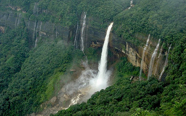
Precipitated water, commonly referred to as rainfall, varies across the land, from near zero (0 mm/yr) in the Atacama desert, in northern Chile (Fig. 19), to close to 12,000 mm/yr in Cherrapunji, Meghalaya, India (Fig. 20). By way of comparison, the mean annual global terrestrial precipitation is about 800 mm, which justifies the classification of climate types shown in Table 1.
|
Regions with climates to the left of the spectrum (arid climates) tend to have their rainfall concentrated in one season, lasting a few months (the wet season), while regions to the right of the spectrum (humid climates) have their rainfall more evenly distributed throughout the year, with no readily identifiable wet or dry season.
|
Components of precipitation
While the amount of rainfall is important in hydrology because it determines environmental moisture and, therefore, the type of climate and vegetation, it is by no means the only relevant parameter. As rainfall hits the ground, it separates into two components: (1) surface runoff, and (2) catchment wetting (L'vovich, 1979). Catchment wetting is defined as the fraction of precipitation not contributing to surface runoff (Ponce and Shetty, 1995a).
In turn, catchment wetting separates into two components: (1) baseflow, and (2) vaporization. Baseflow is the fraction of wetting which exfiltrates as the dry-weather flow of rivers; vaporization is the fraction of wetting which returns to the atmosphere as water vapor. Vaporization consists of three components: (1) evaporation from the ground (the soil and rock mantle), (2) evaporation from bodies of water (wetlands, lakes and reservoirs), and (2) evapotranspiration from vegetation (plants). Deep percolation, the portion of wetting not contributing to either baseflow or vaporization, is a very small fraction of precipitation (a global average of less than 1.5% according to L'vovich, 1979). It is largely intractable and, therefore, usually neglected on practical grounds.
Precipitation has been separated into its three components: (1) surface runoff, (2) baseflow, and (3) vaporization. At first these appear to be in different compartments; the situation in practice is, however, quite different. Surface runoff may join the groundwater through channel infiltration in ephemeral streams. Conversely, baseflow may become runoff through channel exfiltration of perennial streams.
There is some room for confusion in the evaluation of surface runoff. Surface runoff is that which runs directly on the watershed surface (direct runoff), or that which flows as part of a perennial stream, which includes baseflow. In an attempt to clarify the issue, the combination of surface (direct) runoff and baseflow is referred to as streamflow.
Significantly, water that has reached the groundwater table through the action of gravity may return to the atmosphere via: (1) the evaporation of wetlands, or (2) the evapotranspiration of phreatophytes (well plants). The situation is conditioned by geomorphology, which is responsible for the interaction between surface water and groundwater.
On a global average basis, precipitation separates into the following components: (1) evaporation and evapotranspiration, 58%; (2) streamflow, 40%, consisting of direct runoff (28%) and baseflow (12%); and (3) deep percolation (2% or less, considered negligible in practice) (Fig. 21).
|
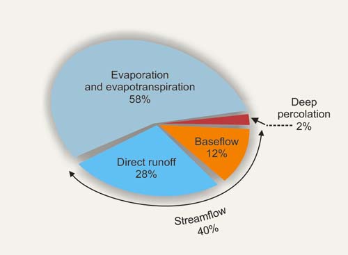
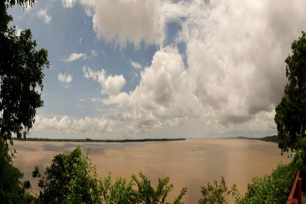
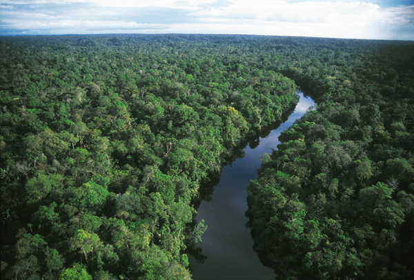
Figure 21 depicts global averages, interpreted at the middle of the climatic spectrum at 800 mm of mean annual precipitation (Table 1). In arid regions, evaporation increases; conversely, in humid regions, streamflow increases. For instance, in the state of Arizona, which is mostly arid, streamflow may account for only about 2% of precipitation. On the other hand, streamflow of the Amazon river at Obidos, a humid basin by any measure, has been determined to be 51% of precipitation (Fig. 22). The runoff coefficient, i.e., the ratio of runoff to rainfall, on a mean annual basis, varies from near 0% in superarid climates to more than 70% in superhumid climates and some geologically unusual locations (L'vovich, 1979).
|
Runoff and not rainfall is what is important from the standpoint of water utilization. Note that on an average global basis, nearly 60% of the precipitation has already been committed to the ecosystems. Of the remaining 40%, i.e., the runoff, a portion of it is reserved for fisheries and other stream biota; so only a small fraction of precipitation may be available for socioeconomic use. The situation is acute in arid regions, where the runoff coefficient may be well below par.
Event versus yield hydrology
The determination of runoff coefficients is subject to an additional complexity: Event and yield runoff coefficients are not the same. The event runoff coefficient C is the ratio of runoff to rainfall for a precipitation event, which typically lasts a short time. On the other hand, the yield runoff coefficient K applies on an annual basis. The difference arises because event water is composed mostly of surface (direct) runoff, while yield water comprises both surface and subsurface (indirect: baseflow) runoff. The different time scales of surface and subsurface runoff determine the difference between event and yield runoff coefficients.
In event hydrology, the runoff coefficient varies from 0 to 1, generally increasing with the degree of imperviousness of the watershed surface (Ponce, 1989). Typical values of C used in urban drainage design are in the range 0.30 ≤ C ≤ 0.70. The lower values apply to undeveloped areas, while the higher values apply to developed areas. Thus, the event runoff coefficient C is directly proportional to the extent of development (as measured by percentage of imperviousness).
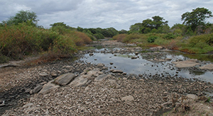
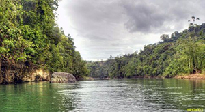
In yield hydrology, the runoff coefficient K varies from 0 to 1, increasing with mean annual precipitation. On the dry side of the climatic spectrum, values of K are typically less than 0.40, and may reach values of zero in cases of extreme aridity (Table 1). Conversely, on the wet side, values of K may reach values of 0.70 or greater. A case in point: L'vovich (1979) has documented values of K ranging from as low as 0.02 (Itapicuru river at Cajueiro, Brazil), to as high as 0.93 (Cayagan river at Pandam, Phillipines) (Fig. 23). Therefore, in yield hydrology, the runoff coefficient K is directly proportional to the prevailing environmental moisture. Additionally, local geology may have an important role in the assessment of yield runoff coefficient.
|
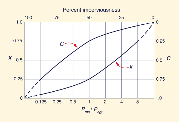
Given the nature of the functional relations governing event and yield runoff coefficients, a schematic model is developed to compare these coefficients across the domain of their variability. Figure 24 shows the yield runoff coefficient K (left scale) as a function of the ratio of mean annual runoff to annual global terrestrial precipitation Pma/Pagt (bottom scale). Concurrently shown is the event runoff coefficient C (right scale) as a function of percent imperviousness (top scale).
|
Conversion of evapotranspiration to runoff
In semiarid regions, conversions of evapotranspiration to runoff have been attempted in the past, with mixed results (Ponce and Shetty, 1995b). The natural ecosystem behaves as a cybernetic system and, therefore, it is not readily subject to analysis using cause-effect relations. Less vegetation may actually translate into less rainfall and less runoff (Ponce et al., 1999). Therefore, conversion of evapotranspiration into runoff may actually be counterproductive in the long run, with both vegetation and runoff being lost under the progressive aridization of the landscape.
Management of groundwater
Surface water (properly, direct runoff) recycles every 11 days on the average, while groundwater may take up to 1,500 years or more (Ponce et al., 2000). In practice, this means that surface water is entirely replenishable in the short run. It may be safely stated that societies will never run out of surface water, because it will be replenished by rainfall sooner or later. The same statement does not follow for groundwater, which typically takes too long to recycle. This poses a relevant question, for which a clear answer is not forthcoming: How much groundwater use is sustainable?
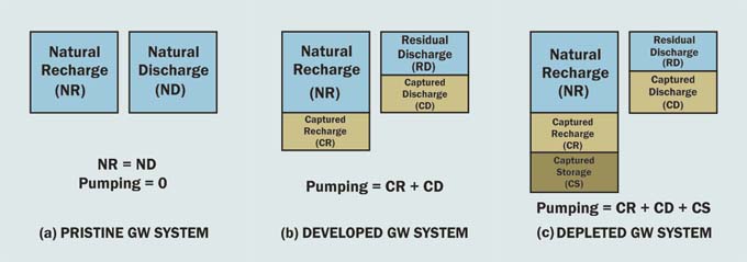
To answer this question appropriately, it is necessary to examine the nature of groundwater flow. All baseflow originates in groundwater; therefore, all groundwater pumping must certainly affect some baseflow in the vicinity. Within a control volume, groundwater pumping amounts to capture (and removal). All capture comes from increases in upstream recharge and decreases in downstream discharge and, in depletion cases, from storage (Fig. 25) (Sophocleous, 1997; Ponce, 2007). To conserve downstream discharge (i.e. baseflow and/or wetland exfiltration), the only sustainable course is to stop well pumping altogether. This, however, imposes an economic hardship on those who, over the years, have made a livelihood from the pumping of groundwater. The solution is to stake a middle ground: To regulate the pumping of the groundwater commons, limiting it to amounts that can be shown not to adversely affect other uses and users in the vicinity (Alley et al., 1999). Pointedly, in this regard, the domain of "vicinity" is a function of the amount of use (Prudic and Herman, 1996).
|
Several studies have revealed a fundamental flaw in conventional hydrogeologic analysis: the assessment of the size of the control volume, which ostensibly serves as the basis for the water balance (Bredehoeft, 1997). The "control volume" in groundwater flow analysis is indeed a moving target; it increases with the amount of pumping (Prudic and Herman, 1996). This is because, unlike surface-water basins, groundwater basins are all connected in their slow but sure quest to reach the nearest ocean by the steepest gradient possible.
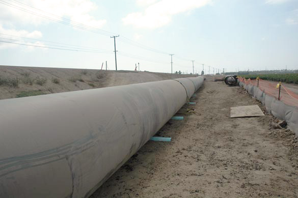
Societies that deplete groundwater are bound to become unsustainable in the long run. Sooner or later they will have to come to grips with the fact that groundwater is not readily recyclable. Tapping deep groundwater for the purpose of developing new (unclaimed) resources may not be the answer either. The salinity content of groundwater is bound to increase with depth, and the disposal of the additional salts brought to the surface may prove to be logistically difficult (Chebotarev, 1955; Ponce, 2012). In peripheral continental regions, brine lines may be built, albeit at great expense, to convey the salts to the ocean, where they can remain forever out of sight and out of mind (Fig. 26).
|
Management of water resources
Vegetation must not be dispensed with in order to tap its water use. Groundwater use should be regulated, because excessive use may lead to resource depletion, not to mention other negative effects (baseflow losses, land subsidence, salinity intrusion, and so on). Additionally, the limited amounts of runoff, particularly in regions on the dry side of the climatic spectrum, must be shared with the native flora and fauna. Therefore, water conservation appears to be the only course for sustainable management.
The import of water from wetter regions, where the supply is plentiful, to drier regions, where the demand is high, is possible, but it may prove to be increasingly difficult, given current environmental, socioeconomic, and political constraints. Desalination of ocean water is also feasible, but it may be sustainable only when used near the low altitude of origin. Excessive pumping of desalinized seawater may lead to an increase in the carbon footprint.
6. ECOLOGY
|
|
Ecology is the science that deals with the interactions between organisms and their environments. The basic unit of ecology is the ecosystem. An ecosystem consists of living (biotic) and non-living (abiotic) components. Living components are the plants, animals, and microbes. Non-living components include the surrounding air, water, and soil and rock. Ecosystems are defined in terms of the study of interactions among organisms and between organisms and their environment.
The force behind ecosystems is the energy from the Sun. Solar energy enters ecosystems through the process of photosynthesis, by which green plants take carbon dioxide from the air and water from the surrounding environment (root zone) to manufacture organic matter in the presence of light. The reaction releases oxygen as a byproduct, which enters the atmosphere. Through respiration, which is the exact biochemical opposite of photosynthesis, animals obtain the energy necessary for their livelihood by burning organic matter (food) using oxygen from the air (for combustion) and releasing carbon dioxide as a byproduct. The atmosphere acts as the reservoir which provides both the carbon dioxide for the plants and the oxygen for the animals. In the process, life of all kinds thrive, all made possible by the energy from the Sun.
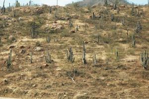
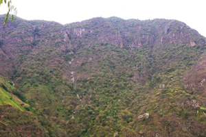
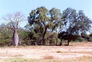
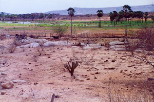
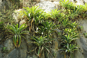
Ecology studies the flora and fauna, and the water, soils, nutrients, and everything else that surrounds them. Depending on the local geology and geomorphology, plants and animals organize themselves in distinct communities, where different species may coexist. A plant community is a collection or association of several plant species within a designated geographical unit or habitat, which forms a relatively uniform patch, distinct from other patches; see, for instance, the two habitats, one semiarid and the other subhumid, both comprised within the La Leche river basin, Lambayeque, Peru (Fig. 27).
|
The components of each plant community are influenced by abiotic factors such as topography, climate, moisture supply, soil type, and disturbance. A plant community may be described either floristically or physiognomically. The floristic description refers to the various vegetative species present in the community. The physiognomic description focuses on the physical structure of the community, its height, canopy density, and specimen size (trunk breast diameter).
While ecology is widely regarded as a subfield of biology, it actually goes beyond the established limits of biology. Ecology encompasses all relations between the three fundamental natural sciences: physics, chemistry, and biology. Ecological knowledge is supported by the earth sciences, including geology, paleontology, geomorphology, climatology, hydrology, hydrogeology, limnology, and oceanography.
The aim of ecology is to describe the relations between living things and their environment. Its fundamental task is the unraveling of the laws of Nature, a high call given the extreme complexity of the processes.
Types of ecosystems
In general, ecosystems are classified according to their domain into: (1) aquatic, (3) transitional, and (3) terrestrial. Aquatic ecosystems can be either: (a) ocean, or (b) freshwater. Transitional ecosystems can be either: (a) longitudinal, or (b) transversal. Terrestrial ecosystems can be either: (a) natural, or (b) artificial.
Specific ecosystems are often referred to as biomes. A biome is a portion of the Earth's surface which is climatically and geographically defined to contain specific communities of flora, fauna, and associated organisms. The different types of biomes are difficult to classify precisely. A tentative classification is shown in Table 2.
| |||||||||||||||||||||||||||||||||
|
Ecological succession
Ecological succession is the observed process of change in the species structure of an ecological community over time. The community begins with relatively few pioneering plants and animals and develops through increasing complexity until it becomes stable or self-perpetuating as a climax community. The engine of succession, the cause of ecosystem change, is the impact of established species upon their own environments.
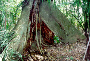
Succession is a process by which an ecological community undergoes more or less orderly and predictable changes following a disturbance or initial colonization of new habitat. Succession may be initiated either by formation of new, unoccupied habitat, such as from a lava flow or a severe landslide, or by some form of disturbance, such as fire, severe windthrow, or logging in an existing community (Fig. 29). Succession that begins in new habitats, uninfluenced by pre-existing communities is called primary succession, whereas succession that follows disruption of a pre-existing community is called secondary succession.
|
Successional change can be influenced by the following factors: (a) site conditions, (b) the character of the events initiating succession (perturbations), (c) the interactions of the species present, and (d) stochastic factors such as availability of colonists, seeds, or weather conditions at the time of disturbance. Some of these factors contribute to predictability of succession dynamics; others add more probabilistic elements. Two important perturbation factors are human activities and climatic change.
Ecological succession has been seen as having a stable end-stage called the climax, shaped primarily by the local climate. This concept has been superseded in favor of nonequilibrium ideas of ecosystems dynamics. Most natural ecosystems experience disturbance at a rate that may make a "climax" community unattainable. Climate change often occurs at a rate and frequency sufficient to prevent arrival at a climax state. Additions to available species pools through range expansions and introductions can also continually reshape communities.
7. ECOHYDROLOGY
|
|
Ecohydrology is the study of ecosystems in relation to the hydrologic cycle. Plants cannot exist without water (the realm of ecology), and water cannot exist without plants (the realm of hydrobiology). Therefore, the question arises: How much water do plants need? Or, conversely, given a region with a certain amount of water, what types of plants are more likely to colonize the region? Note that ecohydrology may be confused with hydroecology, although there is a slight difference in emphasis.
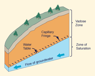
Ecohydrology makes use of concepts of ecology, hydrology, geomorphology, and climatology to develop relations between water and the components of the natural environment. Ecology determines the possible types of biomes. Hydrology determines the amount of available water, in its various forms, including surface water, unsaturated subsurface water (vadose zone) and saturated subsurface water (groundwater) (Fig. 30). Geomorphology uses the force of gravity to relate the existing biomes with the available water, under given spatial and temporal scales. Climatology seeks to explain the spatial relations at the local and regional scales.
|
Water and vegetation: Which comes first?
The different types of biomes on the Earth's surface are closely related to the amount of water and prevailing environmental moisture. The relation is directly proportional: the more water, the more the quantity and diversity of vegetation. A case in point: Average precipitation in the Sahara desert is less than 100-150 mm/yr, while in the Amazon rainforest it is about 2,800 mm/yr.
The supply of moisture stored in the Earth's atmosphere is a function of latitude and climate, varying typically from 2-15 mm in polar and arid regions, to 45-50 mm in humid regions (World Water Balance, 1978). Thus, moisture is 3 to 25 times greater in humid that in arid regions; yet rainfall can be more than 200 times greater! Thus, moisture availability by itself does not explain the amount of rainfall.
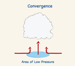
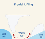
Condensation is very important for precipitation formation. The quickest way for moisture to condense is through cooling, and Nature provides various ways for moisture-laden air masses to cool down. Cooling of air masses is produced by lifting. Three mechanisms for the cooling of air masses are generally recognized: (1) lifting as a result of horizontal convergence, (2) frontal lifting, and (3) orographic lifting. These three processes have a distinct physical flavor. Yet there is a little-known fourth process, which is related to the fact that the Earth's surface emits long-wave radiation, or heat. In many instances, this heat is strong enough to produce lifting of the air masses above it, and consequently, significant amounts of precipitation. Thus, precipitation may be produced: (a) by convergence, particularly in the proximity to a moisture source, (b) through frontal lifting, (c) by air being forced to rise on the windward side of mountains (orographic lifting), or (d) by air being heated from below by long-wave radiation from the Earth's surface (thermal lifting) (Fig. 31).
|
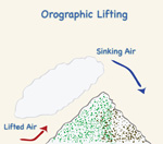
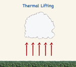
Significantly, humans are unable to alter the course of the first three processes. Latitude determines the amount of lifting and precipitation, but it cannot be changed arbitrarily. Proximity to oceans determines moisture availability, but geographical locations are fixed. The presence of nearby mountains determines lifting, but mountains cannot be moved. One the other hand, humans can have a say on the Earth's surface condition and texture. They can change it at will; in fact, they have been doing just that for the past 10,000 years! Changes from forest to range, from range to agriculture, and from agriculture to urban modify the character of the Earth's surface, altering the long-wave radiation balance.
In thermal lifting, the all-important parameter is albedo. Albedo refers to the property of whiteness, varying in the range 0-1. A value of 0 represents a black body, absorbing all light and eventually releasing the stored energy by emitting heat. Otherwise, the surface will heat up and burn, and the fact that this has not happened through geologic time implies that nearly all of the stored the energy is being returned to the atmosphere. Typically the Earth absorbs light energy during daytime and emits heat during nighttime. We mention "nearly all" because a small percentage, seemingly between 0.1% and 0.3%, is stored in natural vegetation by the process of photosynthesis (Hutchinson, 1970). It is remarkable that such a small percentage is sufficient to sustain all the Earth's ecosystems.
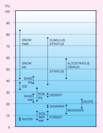
A value of albedo equal to 1 represents a mirror, i.e., an all-reflecting surface. White surfaces, such as freshly fallen snow, have albedos in the range 0.65-0.85. The average albedo of the Earth is 0.15 at the surface and 0.34 at the outer levels of the atmosphere (Fig. 32) (Ponce et al., 1997). The latter value is due to cloud cover; clouds can be of much lighter color than the surface. Now, here is the dichotomy: The albedo of a rainforest is in the range 0.07-0.15, while that of superarid deserts is 0.3-0.6, about four times more. Thus, rainforests will take in more light and release more heat, about four times more on the average, than deserts. Rainforests have an intrinsic means of producing rain by heating the air above. Deserts, on the other hand, lacking sufficient heat from below, are unable to produce lifting, instead producing the opposite effect, subsidence, which hampers rain. That is why deserts are usually cold at night.
|
Since surface albedo determines to a large extent the amount of rain, and green vegetation has a comparatively low albedo, it follows that vegetation produces its own rain. Now, we know from experience that a potted plant needs to be watered every so often for it to grow and flourish. However, the potted plant was not put there by Nature. Where it has placed vegetation, Nature has done it in a cybernetic, self-sustaining way. An ecosystem following a J-curve would have ceased to exist long ago, like the potted plant would if it is not watered. Instead, natural ecosystems follow a biofeedback process, where the cause and effects replace each other regularly, confounding the physical scientist accustomed to the Cartesian mindset of x always being x, and y always being y.
The darker green the ecosystem, the more water it produces; not because the water is there, but because the green is there (Fig. 33). Of course, more water means more green, and more green means more water, confirming the non-Cartesian behavior. This explains why a rainforest may have 50 mm of atmospheric moisture and yet could produce more than 5,000 mm of annual rainfall. [Cherrapunji, in Meghalaya, Eastern India, by most accounts the wettest spot on Earth, averages nearly 12,000 mm of annual precipitation]. On the other end of the climatic spectrum, superarid regions, with about 15 mm of precipitable moisture, may produce hardly any rain at all. [In Northern Chile's Atacama desert, the driest spot on Earth, annual precipitation is about 25 mm, and in some mid-desert spots, rain has never been observed or recorded]. Thus, the ratio of annual precipitation to available moisture in a superhumid region may be much greater than 100, while a comparable ratio for a superarid region may be close to 1.
|
Of all the factors that contribute to the formation of precipitation, none is more subject to anthropogenic alteration than surface albedo. Generally speaking, a decrease in forest areas will lead to less rain. Conversely, an increase in forest areas will lead to more rain. Over the past 10,000 years of human development, the net tendency has been for a decrease.
The role of groundwater
From the standpoint of hydrology, water and moisture exist: (a) on the Earth's surface, (b) in the vadose zone, and (c) in the groundwater. Typically, plants avail themselves of water in the soil, i.e., the vadose zone. Depending on the type of plant, the surface topography, and the proximity of the water table to the ground surface, plants may also be able to tap the groundwater.
By focusing on the plants that tap groundwater, Meinzer (1927) singlehandedly initiated the science of ecohydrology. In the introduction to his seminal work, Meinzer stated:
"... [There are] plants that habitually grow where they can send their roots to the water table or to the capillary fringe immediately overlying the water table and are thus able to obtain a perennial and secure supply of water. These plants have been called phreatophytes. The term is obtained from two greek roots, and it means a "well plant." Such a plant is literally a natural well with pumping equipment, lifting water from the zone of saturation."
Meinzer posed several questions, which are still relevant to this date. We state them here, close to their original form, in the hope of re-energizing much-needed research in the field of ecohydrology.
-
What are the species of phreatophytes?
-
To what extent do these species grow in areas where they cannot reach the zone of saturation?
-
To what extent will other species utilize water from the zone of saturation, and to what extent are they impaired if the water table rises up to their roots?
-
Do phreatophytes develop their root systems in the capillary fringe, or do they send their roots into the zone of saturation?
-
Do phreatophytes manage to avoid the soil's salinity by sending their roots near or into the zone of saturation, where the salinity concentration may be lower?
-
How do phreatophytes adapt to fluctuations in the water table?
-
How are phreatophytes affected by the thickness of the capillary fringe?
-
For a given species of phreatophyte, what is the minimum and maximum depth to the water table that it is adapted to?
-
In species that habitually send their roots to great depths, what adaptations have the young plants developed in order to endure drought until they can get their roots down to the capillary fringe?
-
What is the greatest depth from which groundwater is lifted by plants?
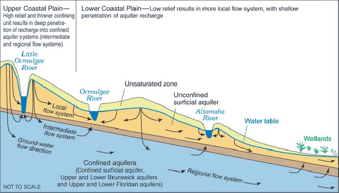
It is clear that plants do rely on the moisture in the vadose zone. It is also clear that some species, particularly the phreatophytes, do rely on the moisture in the capillary fringe and the zone of saturation. Actually, all plants are able to tap at least the capillary fringe, if not the zone of saturation, when the latter are close to the ground surface. How close (how small a distance) will depend on the type of species, and whether their roots, in depth, density, and aerial extent, are able to tap the underlying moisture. Generally, the water table follows the ground surface in a subdued way (Fig. 34). Therefore, the answer to questions of ecohydrology must be found in the related science of geomorphology.
|
The role of geomorphology
Geomorphology is the link between ecology and hydrology. Groundwater is always there, but the actual depth to the water table is determined by climate. In arid regions, the water table may be very deep, while in humid regions it may be very shallow. This is why streams in arid regions are typically ephemeral, with no baseflow, while streams in humid regions are perennial, featuring significant amounts of baseflow.
Meinzer (1927) has aptly described the role of geomorphology, specifically focusing on the arid lands of the western United States. He states:
"... The largest areas of plants that feed on groundwater are in the valley lowlands, but distinctive plants of this group also grow in higher tracts where they are reliable indicators of [the presence of] groundwater. The native plants found in these tracts of shallow groundwater are not the same species as grow elsewhere in the desert, but consist of a few distinctive species which dominate the shallow-water tracts and are absent or have only very sparse growth in other parts of the desert where the water table is not near the surface."
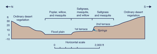
Figure 35 shows the vegetational gradient along a cross section of the Mohave river valley at Camp Cady, California (D. G. Thompson, as cited in Meinzer, 1927). It is seen that different species occupy different steps in the profile. The dimensions of the steps depend on the proximity to groundwater, which is conditioned by the local topography, i.e., by the geomorphology.
|
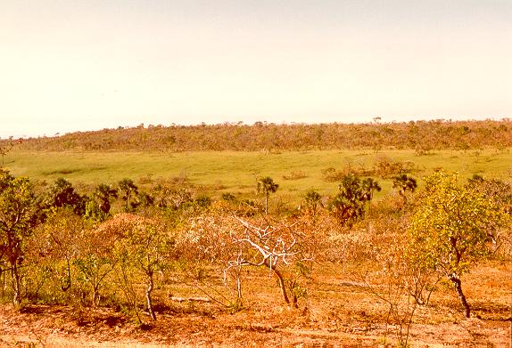
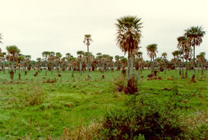
Vegetational gradients of the type shown in Fig. 35 are not restricted to the arid landscapes considered by Meinzer (op. cit.). Figure 36 shows the sequence of cerrado-campo-gallery forest which recurs in the subhumid, highly dissected savannah woodlands of Mato Grosso, in central western Brazil. The cerrado (dense scrub forest) occupies the higher ground, out of reach of the groundwater. The campo (grassland) occupies the middle ground, subject to occasional flooding. The gallery forest occupies the lower ground, where there is a significant and active interaction with groundwater (Ponce and Cunha, 1993 Journal of Biogeography).
|
Categories of plants
Table 3 shows various categories of plants. Plant names are affected with the suffix -phytes, as in halophytes. Table 4 shows a description of the various types of plants that have been identified. Figure 37 shows a sample of the various plants described in Table 4.
|
|
| |||||||||||||||||||||||||||||||||||||||||||||||||||||||||||||||||||
| ||||||||||||||||||||||||||||||||||||||||||
|
8. HYDROCLIMATOLOGY
|
|
Hydroclimatology is the study of the interactions between the hydrologic cycle and the climate. Climate determines precipitation, evaporation, and runoff. Hydroclimatology seeks to describe the relations between climate and the various components of the hydrologic cycle.
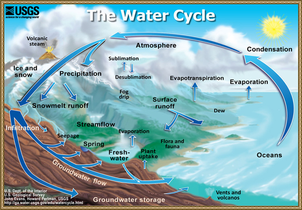
The hydrologic cycle, or water cycle, describes the continuous movement of water on, above, and below the surface of the Earth (Fig. 38). The total amount of water on Earth remains fairly constant over time; yet the partitioning of the available water into the major reservoirs (ice, fresh water, saline water, and atmospheric water) depends on a wide range of climatic variables. The water moves from one reservoir to another, such as from river to ocean, or from ocean to atmosphere. The objective is to study the fluxes and volumes.
|
The conventional approach to the hydrologic cycle is deductive, or Cartesian. The fundamental equation, attributed to Horton (1933), is:
|
Q = P - L | (2) |
in which Q = runoff, P = precipitation, and L = infiltration and other losses.
Equation 2 is strictly applicable to event hydrology. For yield hydrology, an equation similar to Eq. 2 is:
|
Q = P - E | (3) |
in which E = evaporation and evapotranspiration. Equations 1 and 2 are simple, but they are limited because they do not account for interactions between the variables. For instance, Eq. 3 predicts that the larger the evapotranspiration, the smaller the runoff. Yet there are some situations in Nature where the converse may be true: the larger the evapotranspiration, the larger the runoff, particularly in view of climate change.
Further proof that Eq. 2 fails to account for all the relevant processes is the NRCS runoff curve number equation, which is well established in urban hydrology (Ponce and Hawkins, 1996). This equation, developed by Victor Mockus (Ponce, 1996), is based on the assumption of proportionality between retention and runoff, such that the ratio of actual retention to potential retention is equal to the ratio of actual runoff to potential runoff:
|
P - Q Q _______ = ____ S P | (4) |
in which S = potential retention. This equation predicts that the greater the retention, the greater the runoff, a conclusion which is in conflict with Eq. 2.
A significant deficiency of Eq. 3 is that it may lead to double-counting in the water balance. If the hydrologic abstractions are interpreted as infiltration, as is usually the case, the latter could follow one of two paths, either: (1) return to the atmosphere as evaporation and evapotranspiration (of vegetation, soil moisture, and wetlands), or (2) percolate down to join the groundwater, eventually appearing as runoff (baseflow) somewhere downstream. The double counting is because the same volume of water is being counted as hydrologic abstractions and as runoff.
The conventional analysis of the water balance is improved by the cybernetic (feedback) approach pioneered by Budyko and Drozdov (1953), complemented with the work of L'vovich (1979). Budyko and Drozdov (1953) used a hydroclimatological model of a coupled land surface-atmosphere system to study the components of the hydrologic cycle. L'vovich (1979) introduced the concept of catchment wetting, thereby eliminating the double counting in the water balance.
Budyko's hydroclimatological model
The annual water balance for an exorheic basin may be expressed as follows:
|
ΔS = P - E - Q | (5) |
in which ΔS = change in basin storage, P = precipitation, E = evaporation, and Q = total runoff, consisting of surface runoff and groundwater runoff. The basin storage consists of surface, subsurface, and groundwater storage.
In an average year, ΔS = 0, and Eq. 5 reduces to:
|
P = E + Q | (6) |
where the values in Eq. 6 now represent mean annual values.
Equation 6 assumes that deep percolation, i.e., the groundwater runoff that discharges directly into the ocean, bypassing the surface runoff, is negligible. On a global basis, L'vovich (1979) has calculated that deep percolation is about 5% of runoff, while the latter is approximately 30%-40% of precipitation. Thus, in general, only a small fraction of precipitation (less than 2%) infiltrates deep enough into the ground to bypass the surface waters altogether.
Budyko assumed a control volume comprising the land surface-atmosphere system shown in Fig. 39. In this figure, A is the water vapor entering the atmosphere horizontally, through advection, and E is the water vapor entering the atmosphere vertically, through evaporation from the land (the combined evaporation from land surface, water bodies, and vegetation).
|
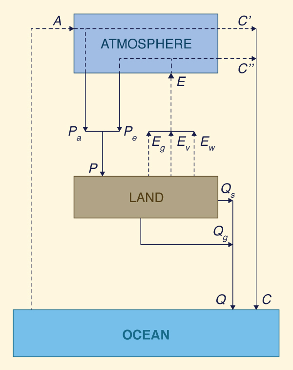
Precipitation P may be separated into two components:
|
P = Pa + Pe | (7) |
in which Pa = fraction of P derived externally, from A; and Pe = fraction of P derived internally, from E.
From conservation of mass:
|
A = C + Q | (8) |
in which C = total water vapor exiting the control volume at the leeward side. Furthermore:
|
C = C' + C" | (9) |
in which C' = water vapor in transit, defined as follows:
|
C' = A - Pa | (10) |
subject to C' ≥ 0.
The quantity C" = water vapor discharge, i.e., the fraction of evaporated water that does not recycle and, instead, leaves the control volume at the leeward side, defined as follows:
|
C" = E - Pe | (11) |
subject to C" ≥ 0.
Budyko assumed that P and E are spatially averaged over the control volume. The advected water vapor at the windward side is WU, where W is the moisture content (m) of the atmospheric column and U is the mean velocity (m/s) of the input advected water vapor. For simplicity, assume a linear decrease in advected water vapor as the moist air moves across the region. The corresponding flux at the leeward side is: WU - PaL, where L = length measure of the control volume, taken as the square root of the area of its vertical projection. Thus, the external water vapor flux, spatially averaged over the control volume, is: WU - 0.5 PaL.
The internal water vapor flux at the windward side of the control volume is zero; the
corresponding flux at the leeward side, assuming a linear increase as the moist air moves
across the region, is:
The atmosphere is assumed to be completely mixed; therefore, the ratio of externally to internally derived precipitation is equal to the ratio of spatially averaged external to internal water vapor fluxes.
|
Pa WU - 0.5 PaL ______ = _________________ Pe 0.5 (E - Pe) L | (12) |
which through algebraic manipulation reduces to:
|
Pe = Ω Pa | (13) |
where Ω is a dimensionless climatic parameter defined as (Entekhabi et al., 1992):
|
EL Ω = _______ 2WU | (14) |
From Eqs. 7 and 13:
|
P Pa = _______ 1 + Ω | (15) |
and
|
ΩP Pe = _______ 1 + Ω | (16) |
When Pa is small compared to P, Ω is large and effective precipitation recycling is taking place. Conversely, when Pa is large compared to P, Ω is small and little recycling is taking place. Thus, Ω is directly related to the precipitation recycling capacity of the coupled land surface-atmosphere system.
Values of Ω ranging from 0.02 (Antarctica: inner continental region), to 0.05 (Australia: Pacific Ocean drainages), to 0.34 (North America: Atlantic Ocean drainages), to 0.68 (South America: whole continent) have been documented in World Water Balance (1978). Low values of Ω (0.02-0.10) indicate a hyperarid-arid climate, average values (0.15-0.30) a semiarid-subhumid climate, and high values (0.40-0.60) a humid-perhumid climate.
The evaporation originates from three different sources (Fig. 38):
|
E = Eg + Ev + Ew | (17) |
in which Eg = evaporation from bare ground; Ev = evaporation from vegetated surfaces (evapotranspiration), and Ew = evaporation from water bodies. The fate of evaporation is either to recycle as Pe or to exit the control volume as water vapor discharge C" (Fig. 38).
Equations 15 and 16 were derived assuming a linear change in water vapor fluxes as the moist air is transported
across the control volume. This limits the applicability of these equations to regions with
Relation with albedo
The lower albedos associated with open water, vegetation, and moist land surfaces make possible the increased absorption of solar and long-wave radiation, resulting in increased evaporation and greater environmental moisture. Therefore, albedo is intrinsically related to environmental moisture. In turn, environmental moisture is directly related to Ω and to the moisture-recycling capacity of the coupled land surface-atmosphere system.
Greater environmental moisture implies that the source of most of the evaporation is
(Ev + Ew), which is typical of a humid region.
Conversely, lesser environmental moisture implies that the source of most of the evaporation is Eg,
which is typical of an arid region. Thus, a lower albedo would correspond to a higher (Ev + Ew) / E ratio,
while a higher albedo would correspond to a higher
Several studies have documented the relation between environmental moisture and the recycling capacity of the coupled land surface-atmosphere system. Benton et al. (1950) estimated that the portion of precipitation derived from local evapotranspiration for the Mississippi river valley was at most 10%. The same percentage was estimated by Budyko and Drozdov (1953) for the European portion of the former USSR. In the humid Amazon basin, Salati et al. (1979) and Salati and Vose (1984) have measured a recycling rate of 48%, while Lettau et al. (1979) have found the 88.4% of the total amount of rain at 75°W longitude (in the Amazon basin) falls at least a second time.
In some instances, anthropogenic influence on the moisture recycling capacity may be substantial. For instance, Stidd (1975) has reported that evapotranspiration from irrigation development in the Columbia river basin was recycled at least once as rainfall. Moreover, Balek (1983) has stated that an increase in annual rainfall of 5-10% in the vicinity of Kariba dam, in Africa, was traceable to increased evaporation after the establishment of the reservoir.
Water balance coefficients
Budyko's hydroclimatological model enables the definition of three water balance coefficients:
|
Pe Kc = _____ P | (18) |
|
C" Kd = _____ P | (19) |
|
Q Kr = _____ P | (20) |
Given Eqs. 6 and 11, it follows that:
|
Kc + Kd + Kr = 1 | (21) |
Table 5 shows the application of Budyko's model for selected values of mean annual
precipitation
| |||||||||||||||||||||||||||||||||||||||||||||||||||||||||||||||||||||||||||||||||||||||||||||||||||||||||||||||||||||||||||||||||||||||||||||||||||||||||||||||||||||
Figure 40 shows the variation of water balance coefficients across the climatic spectrum. The cycling coefficient Kc is directly related to mean annual precipitation; therefore, the greater the environmental moisture, the greater the recycling capacity of the coupled land surface-atmosphere system. The discharge coefficient Kd is inversely related to mean annual precipitation; i.e., arid regions have a greater capacity for water vapor discharge than humid regions. The runoff coefficient Kr is directly related to mean annual precipitation; i.e., the greater the environmental moisture, the greater the runoff coefficient. This latter conclusion has been validated by experience (L'vovich, 1979).
|
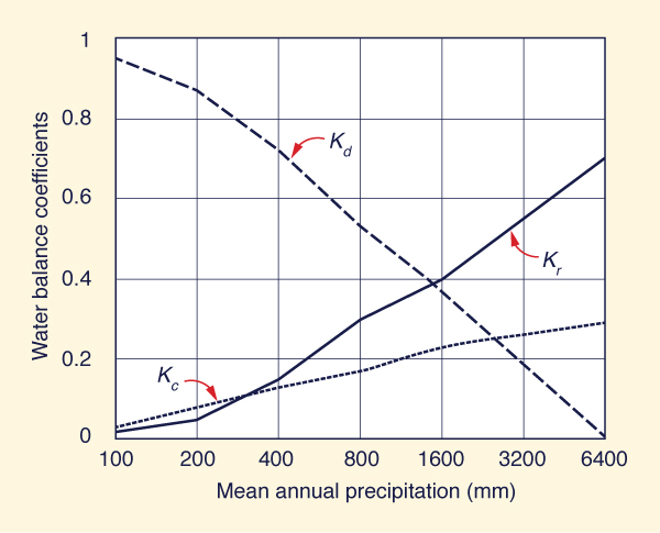
Note that the most significant changes in water balance coefficients seem to occur around the middle of the climatic spectrum, where a large fraction of the human population resides. Therefore, anthropogenic changes in albedo may be particularly crucial in semiarid and subhumid regions, from 400 to 1600 mm of mean annual precipitation.
Catchment wetting
On a global basis, precipitation goes into two compartments: (1) vaporization (evaporation and evapotranspiration), and (2) runoff (streamflow) (Fig. 21). The conventional water balance separates precipitation into: (1) losses, and (2) runoff (Eqs. 2 or 3). Yet a portion of the losses, of which infiltration is a significant fraction, eventually shows up as baseflow, adding to streamflow. Hence, the double counting.
The problem has been solved using the concept of catchment wetting, developed by L'vovich (1979). L'vovich separated annual precipitation into two components (Fig. 41):
|
P = S + W | (22) |
in which S = surface runoff, i.e., the fraction of runoff originating on the land surface, and
|
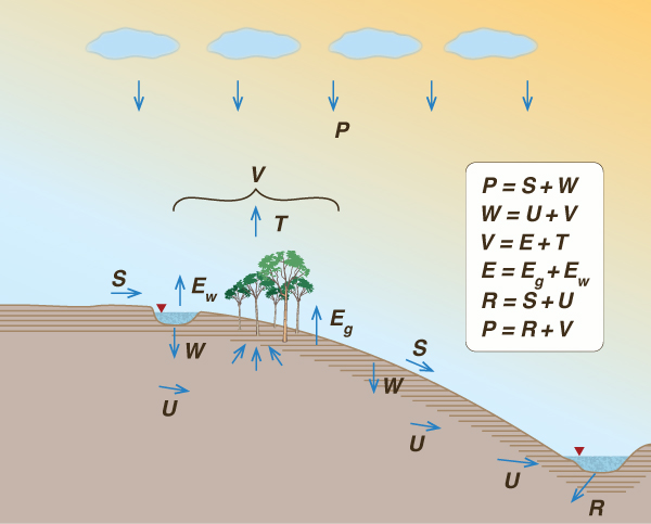
Wetting is separated into two components:
|
W = U + V | (23) |
in which U = baseflow, i.e., the fraction of wetting which exfiltrates as the dry-weather flow of streams and rivers, and V = vaporization, i.e., the fraction of wetting returned to the atmosphere as water vapor. [L'vovich's model neglects deep percolation, the portion of wetting which bypasses the surface waters altogether, estimated at less than 2% of precipitation on a global basis].
Vaporization, which comprises all moisture returned to the atmosphere, has two components:
|
V = E + T | (24) |
in which E = nonproductive evaporation, hereafter referred to as "evaporation," and T = productive evaporation, i.e., that resulting from plant transpiration, hereafter referred to as "evapotranspiration."
Evaporation has two components:
|
E = Eg + Ew | (25) |
in which Eg = evaporation from the ground, bare soil, and small surface storage (puddles), and Ew = evaporation from water bodies such as lakes, reservoirs, streams, and rivers.
Evapotranspiration is the evaporation from vegetated surfaces such as leaves and other parts of plants, a function of the physiological need of plants to pump moisture from the soil to maintain turgor and avail themselves of nutrients.
Runoff (i.e., total runoff) is the sum of surface runoff plus baseflow. Therefore:
|
R = S + U | (26) |
Combining Eqs. 22, 23, and 26:
|
P = R + V | (27) |
Equations 22 to 27 constitute a set of water balance equations. Combining Eqs. 26 and 27 leads to:
|
P = S + U + V | (28) |
Equation 28 separates annual precipitation into its three major components: (1) surface runoff, (2) baseflow, and (3) vaporization. Significantly, Eq. 28 assumes that the change in soil-moisture storage from year to year is negligible, an assumption which is useful as a first approximation.
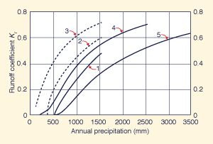
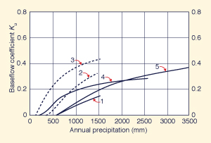
Given Eqs. 22 to 27, two water balance coefficients may be defined: (1) runoff coefficient, and (2) baseflow coefficient. The runoff coefficient is:
|
R R Kr = _____ = __________ P R + V | (29) |
The baseflow coefficient is:
|
U U Ku = _____ = __________ W U + V | (30) |
Figure 42 shows runoff and baseflow coefficients calculated by Ponce and Shetty (1995b), based on data reported by L'vovich (1979). It is seen that in all cases, runoff and baseflow coefficients increase with annual precipitation.
|
|
Outlook
It is clear that surface runoff, baseflow, and vaporization (Eq. 28) vary across the climatic spectrum. Albedo is the fundamental parameter of hydroclimatology; lower albedos lead to rainforests, while higher albedos lead to deserts. Anthropogenic modifications of albedo (conversions of forest to range, range to agriculture, and agriculture to urban) are bound to produce changes in albedo, which will generally have the effect of lowering precipitation and decreasing surface runoff. However, in some instances, extensive irrigation and large storage reservoirs may actually reduce albedo, which will have the beneficial effect of increasing precipitation.
9. BIOCLIMATOLOGY
|
|
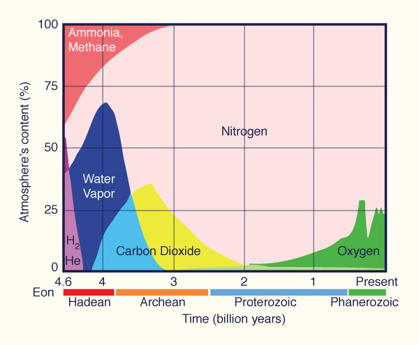
Bioclimatology is the study of the seasonal and long-term relations between the Earth's biosphere and atmosphere. Since the beginning of time, these two spheres have interacted with each other in the presence of water (the hydrosphere) and soil and rocks (the lithosphere). The primordial atmosphere was nearly devoid of oxygen (Fig. 43). After nearly 3 billion years of photosynthesis, the oxygen level of the atmosphere is now close to 21%, a level appropriate to sustain the fauna that developed over the past 600 million years (Cloud and Gibor, 1970). The plants could not develop without water, and the required nutrients came from the soil and rock. Thus, the interaction of the four spheres made possible the ecosphere, the sum total of all ecosystems of Earth.
|
Climate and ecosphere interact with each other in a myriad of ways. The system is self-controlled, cybernetic, with the specific aim of self perpetuation. Climate controls the distribution and characteristics of all living organisms. Global and mesoscale atmospheric currents control the amount of precipitation. In turn, the latter determines which organisms are naturally adapted to survival.
Bioclimatology seeks to study what type of organisms develop under what climate. The task is complex because climate varies with several environmental factors, among which are: (1) mean annual precipitation, (2) potential evapotranspiration, (3) latitude, and (4) altitude. In turn, potential evapotranspiration is a function of: (1) temperature, (2) relative humidity, and (3) wind speed. Temperature is a function of: (1) latitude, (2) altitude, and (3) continental location relative to the nearest ocean.
Seeking to simplify what amounts to a very complex process, Holdridge (1947) reduced the climatic parameters to: (1) (mean) annual precipitation, (2) potential evapotranspiration ratio (the ratio of potential evapotranspiration to mean annual precipitation), and (3) biotemperature, the latter intended to reflect the combined effect of latitude and altitude (Fig. 44). Biotemperature is based on the growing season length and temperature. For a specific site, it is determined by adding the average mean monthly temperatures greater than 0°C, and dividing by 12.
|
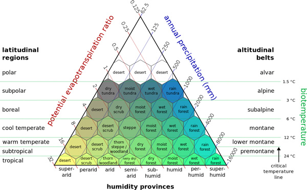
For a specific site, the precipitation is the mean annual precipitation (mm). Note that Holdridge used a mean annual precipitation of 1,000 mm as the middle of the climatic spectrum (the center of the humidity provinces), unlike in Table 1, where this value is taken as 800 mm. In Fig. 44, the temperature and precipitation values determine a point which falls within a hexagon representing a biome. When the point falls within one of the border triangles of a hexagon, the vegetation of that area will show a transitional character, i.e., an ecotone.
All altitudinal belts will be found only in the tropics. In other latitudinal regions, only the altitudinal belts above the basal formations for the region will be found. The ranges of altitudinal belts are approximately the following: alvar (or nival), undefined; alpine, 500 m; subalpine, 500 m; montane, 1,000 m; and lower montane, along with the subtropical, if present, 2,000 m. The tropical basal regions vary from 0 to 1,000 m; the warm temperature alone or with the low subtropical, 0-2,000 m; and the basal formation of the other regions, from 0 m to the maximum for the corresponding belt.
In Holdridge's classification, the latitudinal regions are divided into: (a) tropical, (b)
subtropical,
|
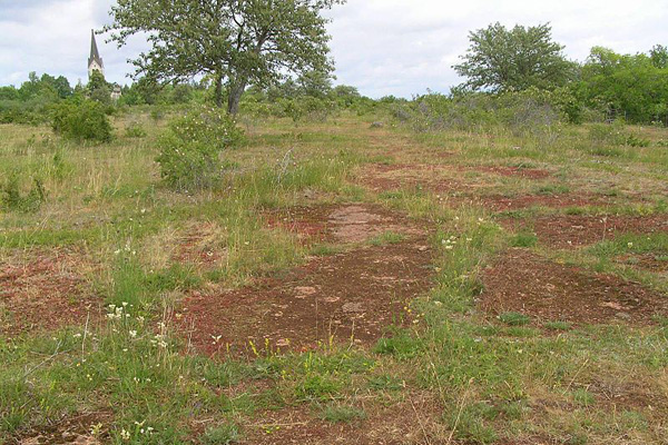
Alvars are vegetative communities founded on exposed bedrock (Fig. 46). This stressed habitat supports a community of rare plants and animals, including species more commonly found on prairie grasslands. Lichen and mosses are common species; trees and bushes are absent or severely stunted.
|
Bioclimatological indexes
Temperature varies not only with latitude and altitude, but also with continental location relative to the nearest ocean. Three temperature indexes are used to study bioclimatological relations: (1) continentality index; (2) thermicity index, and (3) positive temperature index (Rivas-Martínez, 2007):
- Continentality index
This index is equal to the average temperature of the hottest month Thot minus the average temperature of the coldest month Tcold .
Ic = Thot - Tcold
(31) The following procedure is used to calculate Thot :
The maximum daily temperature, for each month and year of record is identified, and the mean maximum monthly temperature is calculated.
The mean of the mean maximum monthly temperature is calculated for the entire record.
The month with the highest mean of the mean maximum monthly temperature is selected as the hottest month.
A similar procedure is applied to calculate Tcold.
The continentality index varies between Ic = 0 for an extreme oceanic influence, to Ic = 65 for an extreme continental influence. Table 6 shows the classification of climates as a function of the continentality index.
Table 6. Classification of climates based on continentality index. Types Continentality index Ic Hyperoceanic 0 - 11 Oceanic 11 - 21 Continental > 21
- Thermicity index
This index is equal to the mean annual temperature Tmean plus the mean of the monthly minimum temperatures Tmin plus the mean of the monthly maximum temperatures Tmax. The sum is multiplied by 10.
It = 10 (Tmean + Tmin + Tmax)
(32) The mean annual temperature is the mean of the (12) mean monthly average temperatures. The mean of the monthly minimum temperatures in the mean of the (12) mean monthly minimum temperatures. The mean of the monthly maximum temperatures in the mean of the (12) mean monthly maximum temperatures.
- Positive temperature index
This index is equal to the sum of all positive (nonnegative) mean monthly temperatures. The sum is multiplied by 10.
Tp = 10 ( ∑ Tpos )
(33) Table 7 shows the classification of climates as a function of the thermicity and positive temperature indexes.
Table 7. Classification of climates based on thermicity
and positive temperature indexes.Type of climate Thermicity index It Positive temperature index Tp Infratropical 710 - 890 2900 - 3700 Thermotropical 490 - 710 2300 - 2900 Mesotropical 320 - 490 1700 - 2300 Supratropical 160 - 320 950 - 1700 Orotropical 120 - 160 450 - 950 Criorotropical 225 - 450
10. ECOHYDROCLIMATOLOGY
|
|
Ecohydroclimatology is the study of the interactions between ecology, hydrology, and climate. Ecology refers to the ecosystems, i.e., the flora and fauna adapted to a given region, hydrology refers to the various volumes and fluxes in the water cycle, and climate refers to the mean properties of the atmosphere. Actually, the lithospere is also present in the interaction, although not explicitly mentioned.
The fundamental aim of ecohydroclimatology is the unraveling of the interactions between plants, water, geology/geomorphology, and climate. Plants increase in density and species diversity with environmental moisture, i.e., the humidity provinces (Fig. 44). Water exists in the terrestrial environment as: (a) surface water, (b) vadose zone moisture, and (c) groundwater.
Groundwater volumes exceed surface-water volumes by about two orders of magnitude (Fig. 47). Therefore, there is an abundance of groundwater as compared to surface water. Yet groundwater differs from surface water in one very important respect: while surface water recycles readily, groundwater does not. Surface water cannot be depleted, while groundwater can.
|
Surface water is generally fresh; however, the salinity of groundwater increases with depth (Ponce, 2012). Hydrodynamic and hydrochemical gradients affect the distribution and type of groundwaters. Chebotarev (1955) has identified three hydrodynamic zones in groundwater flow (Fig. 48):
- Zone of active exchange,
- Zone of delayed exchange, and
- Zone of stagnant conditions.
|
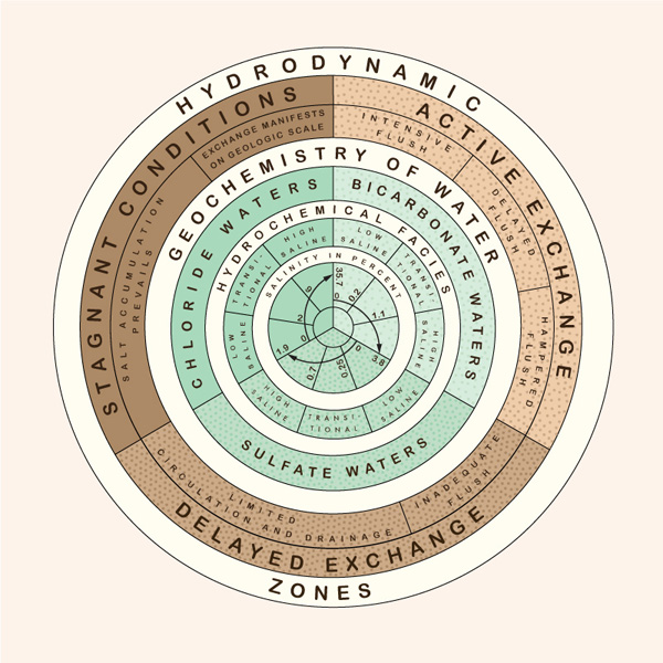
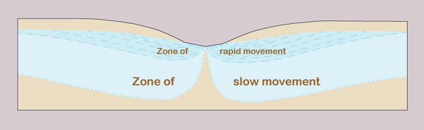
The type of exchange, or replenishment rate, is inversely related to the detention time, i.e., locally,
the ratio of volume to discharge. Small hydrodynamic gradients lead to low velocities and small discharges
and, consequently, to long detention times. The increase in salinity concentration becomes apparent as
the exchange rate changes from active to delayed and eventually to stagnant conditions.
Therefore, zones of smaller gradients and slower movement occur in deeper strata
|
Pumping groundwater at great depths may have the unintended consequence of bringing large quantities of salt to the surface, where they would have to be disposed of properly, usually at great expense. Therefore, caution is recommended when pumping groundwater at great depths, particularly for consumptive uses such as irrigation.
Aquifers are of two types: (1) sedimentary (alluvial), and (2) fractured rock; for instance, compare the spatial distribution of aquifers in the Australian continent (Fig. 50). Sedimentary aquifers differ from fractured rock aquifers in two respects: (1) their greater storage capacity (specific yield), and (2) their slower rate of replenishment. Aquifers may also be classified as: (1) unconfined, and (2) confined. Unconfined aquifers are at atmospheric pressure, while confined aquifers are typically above atmospheric pressure.
|
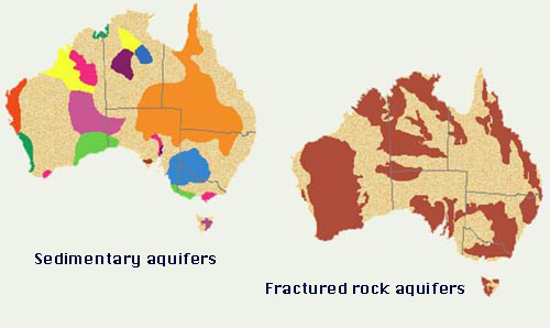
Most plants get their water from the vadose zone (Fig. 30). The extent of the vadose zone depends of soil texture or rock type. The amount of moisture in the vadose zone depends on the humidity province: It is less in arid regions and more in humid regions.
Some plants are able to get their water directly from the groundwater, or else, from the capillary fringe ling directly above it. Groundwater exists everywhere in the soil and rock mantle, deeper in arid regions and shallower in humid regions. Therefore, the distribution of plants of the Earth' surface is determined by:
Position along the climatic spectrum of environmental moisture, as described by the humidity provinces (Fig. 44),
Depth to the water table, which determines whether the plants can avail themselves of moisture in the capillary fringe or the groundwater beneath it, and
The presence/absence of springs, which depends heavily on the local geology and geomorphology.
Figure 51 shows a riparian corridor of coast live oak (Quercus agrifolia) in Tierra del Sol, San Diego County, California. The creek is ephemeral, with surface water flowing only in response to rainfall. Yet there is enough year-round moisture in the soil to support a healthy riparian corridor.
|

Depending on the local geology and geomorphology, springs may flow into wetlands, enabling the support of significant amounts of vegetation. For instance, Fig. 52 shows a very large specimen of coast live oak located in the McCain ranch, McCain valley, Boulevard, San Diego County, California. The specimen, measuring 7.55 m in circumference at breast height, is estimated to be at least 300 years old. The absence of this type of vegetation in the rest of McCain valley strongly indicates that this community of coast live oak is being sustained by groundwater from local springs (Ponce, 2013).
|
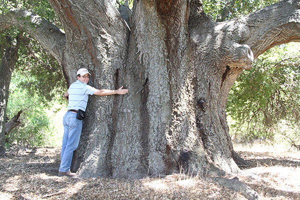
All landscapes are subject to dissection by streams and rivers. Uplift and erosion determine the extent to which a certain landscape is dissected. Soil type also has a bearing in the extent of dissection. For a given landscape and humidity province, geomorphology determines how deep is the water table. Thus, geomorphology has a major role in determining the extent to which plants can tap groundwater.
Climate conditions the regional aspect of vegetation; geomorphology conditions the local aspect. Vegetative communities organize themselves into ecosystems and biomes, defined, first, by the prevailing climate and, secondly, by the underlying geomorphology. The differences in elevation do not need to be substantial; in some instances, two different species may colonize patches that are only a few centimeters apart in elevation.
The importance of geomorphology in ecohydroclimatology is tempered by two factors:
Degree of dissection, as expressed by drainage density, and
Overall slope of the terrain.
Drainage density conditions runoff; generally, the higher the density, the faster and greater the runoff, and vice versa.
An example of high drainage density is the Chinle Badlands, in the
Grand Staircase-Escalante National Monument, Utah
|
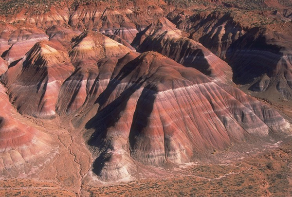
|
The overall slope of the terrain is a second key parameter. Terrain slopes vary widely, from very steep
to very mild. For instance, some hillslopes of
the La Leche river basin, in the Western Andes range, Lambayeque, Peru,
exceed 45% [Fig. 55 (a)]
(Ponce, 2008).
On the other extreme, the Pantanal of Mato Grosso, in Brazil, the largest wetland in the world,
features terrain slopes of about 0.001%
|
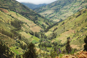
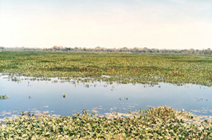
The flatter the terrain, the more the longitudinal and transversal runoff diffusion and
consequent spreading of the flows onto increasingly larger areas.
The phenomenon is admirably described by unsteady open-channel hydraulics.
Combining the equations of water continuity and motion (neglecting the inertia terms) results in a second-order partial differential
equation describing the convection (translation) and diffusion (attenuation) of a given discharge (Ponce, 1989):
|
∂Q dQ ∂Q Qo ∂2Q ______ + ( ______ ) ______ = ( _________ ) _______ ∂t dA ∂x 2 T So ∂x2 | (34) |
The convective velocity is the
kinematic wave celerity (Seddon, 1900; Lighthill and Whitham, 1955):
|
dQ ck = ______ dA | (35) |
The diffusion coefficient is the
hydraulic diffusivity (Hayami, 1951; Ponce, 1989):
|
Qo qo νh = _________ = _______ 2 T So 2 So | (36) |
From Eq. 36, the diffusion coefficient is seen to be inversely proportional to slope. Thus, large slopes lead to negligible diffusion, while mild slopes lead to very strong diffusion. Diffusion causes the spreading of the flows, affecting the ecohydrological and hydroclimatological relations.
Kinematic slopes, greater than 1%, do not diffuse, with the water exiting the land as fast as possible and becoming part of runoff and, therefore, not part of evapotranspiration (Ponce, 1989). On the other hand, for dynamic slopes, i.e., those less than 0.01%, the flow diffuses, spreads out onto the land and the water stands a better chance of converting into evapotranspiration.
In tropical/subtropical ecology, the seasonal/annual flood pulse, which sustains the aquatic-terrestrial transition zone (ATTZ), owes its existence to the mild channel slopes that are generally present in large basins such as the Upper Paraguay (Fig. 56) (Junk et al., 1989).
|
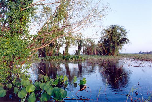
In summary, drainage density, terrain slope, depth to the water table, and the presence/absence of springs, are all geomorphological factors which interact with each other to determine ecohydrological and hydroclimatogical relations. Ecohydroclimatology arises from them.
11. CASE STUDIES
|
|
Several case studies of ecohydroclimatology are reviewed. It is shown how geomorphology has a leading role in characterizing the interactions between flora, fauna, water, and climate. Examples of anthropogenic interaction are also noted.
A. The savannah vegetation of Brazil
Cole (1960), in her seminal paper on the distribution and origin of the savanna vegetation of Brazil, recognized the importance of the dynamic nature of vegetation and its relation to landscape evolution and climate change. In the conclusion, she states the following:
"The distribution of the grassy savanna, caatinga [thorn woodland] and mata [moist forest] is thus explained in terms of the ages of their respective floras and the geomorphological evolution of the landscape. The exact distribution at any given period of time is related to the stage in the cycle of erosion, with the campo cerrado [grassy savanna woodland] representing an edaphic climax on the level plateaus and the mata a climatic climax on those lands which have been given an adequate drainage and good soils as a result of dissection in the current cycle... The dynamic nature of the situation, however, must be appreciated. All the time the surface features are being modified by the agents of erosion and deposition. And all the time successional and migrational changes are taking place in the vegetation cover with a general tendency for an extension of the mata and the caatinga at the expense of the campo cerrado and other grassy savannas... Periods of increased dissection, either associated with a wetter climate or following continental uplift, will favor the extension of forest, whereas increased aridity will lead to the spread of caatinga, and long periods of stability leading to vast pediplains and wornout soils will favor grassy savannas in the wetter areas and caatinga scrub in the arid ones."
Cole (op. cit.) stresses the importance of geology and geomorphology in a matrix of dynamic change, where floras (usually belonging to two contiguous humidity provinces) compete for the available resources. In many instances, and sometimes without full knowledge, humans interfere with these natural processes, producing an accelerated change in one direction or another.
A striking example of Cole's argument for vegetative competition in a geomorphological setting is given by the earthmounds populating the floodplain of the Araguaia river, in Mato Grosso, Brazil (Smith, 1971). When viewed from the air, the striking spatial regularity of the earthmounds defies comprehension (Fig. 57).
|
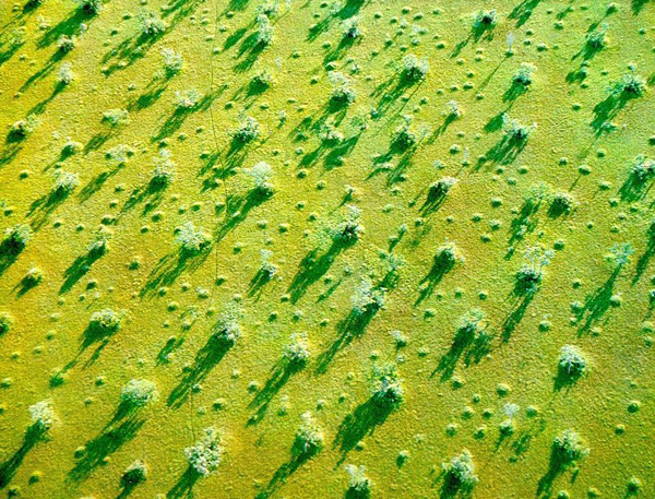
B. The Pantanal of Mato Grosso, Brazil
The Pantanal of Mato Grosso is the largest tropical wetland in the world, encompassing about 140,000 km2 in Mato Grosso and Mato Grosso do Sul, Brazil, with smaller portions in northern Paraguay and eastern Bolivia. The wetland is located wholly within the Upper Paraguay river basin.
The ecohydrological setting of the Upper Paraguay river basin and the Pantanal of Mato Grosso is unique in the American continent. The basin is strategically located contiguous to four major South American biomes, which surround it, exerting their influence on it (Ponce, 1995) (Fig. 58):
The humid Amazon rainforest to the north and northwest,
The subhumid savanna woodlands (cerrados) of Central Brazil to the northeast, east, and southeast,
The humid Atlantic forest to the south, and
The semiarid scrub forest (Chaco) of Eastern Bolivia and Northwestern Paraguay to the west and southwest.
|
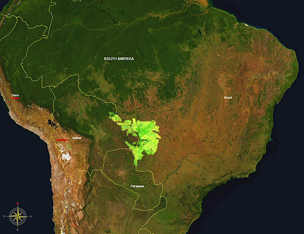
The unusual combination of geology, geomorphology, and hydrology has contributed to the richness and variety of the Pantanal vegetation. In turn, this helps sustain a diverse group of ecosystems, where a complex assortment of permanent swamps, seasonal swamps, and terra firma is seasonally replenished with ample moisture, sediment, and nutrients (Fig. 59). The entire process hinges on the high rate of vaporization (estimated at 92%) which characterizes the hydrologic budget of the Upper Paraguay river basin (Ponce, 1995).
|
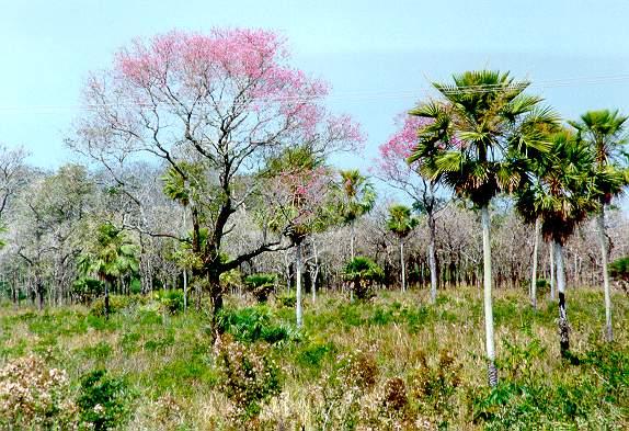
In the existing literature, the Pantanal vegetation is often marked as a single unit and referred to as the "Pantanal" complex. Actually, the latter is a mosaic of many different communities, with frequent abrupt changes often correlated with topography, and many ecotones. The Pantanal has no endemic flora of its own; rather, it is made up of elements from mata (deciduous and semideciduous forests transitional to the tropical Amazon rainforest and the humid Atlantic forest), campo (open grassland), cerrado (savanna woodland), and caatinga (desert scrub forest).
The most striking aspect of the Pantanal is its curious combination of mesic and xeric vegetation growing side by side, a result of its unique combination of climate and geomorphology (Tricart, 1982). Toward the center of the Pantanal, the climate is markedly seasonal, with a clearly defined drought period. Given the extremely flat topography, a small difference in elevation (1 to 2 m, or less) is all that is needed to make a great difference in seasonal soil moisture, particularly when the underlying strata is coarse alluvium.
Prance and Schaller (1982) and Schaller (1983), among others, have noted the strong cerrado element in the Pantanal. These cerrados are dominated by species such as Bowdichia virgiloides, Caryocar brasiliense, Curatella americana, Qualea parviflora, and Tabebuia caraiba, which are typical of the savanna woodlands of Central Brazil. Cerrado occurs mainly in the nonflooded upland, but also towards the eastern edge of the Pantanal, where the land is inundated for only short periods at the height of the flood season. Such wet cerrado tends to consists of numerous islands of cerradão (dense cerrado forest) on slightly elevated areas that are not flooded.
Cerrado tree species which are most resistant to waterlogging (e.g., Byrsonima crassifolia and Curatella americana) are common near the boundary cerrado/campo, and on raised islands of ground in wet campos (Furley and Ratter, 1988). The distribution of these islands produces the campos de murundus, consisting of an expanse of wet campos dotted with a regular pattern of raised earthmounds bearing cerrado trees, shrubs, and often termitaria. The larger earthmounds, or capões, are circular or elliptical in shape, of lengths up to 300 m, and sparsely distributed across the seasonally flooded campos (Ponce and Cunha, 1993) (Fig. 60).
|
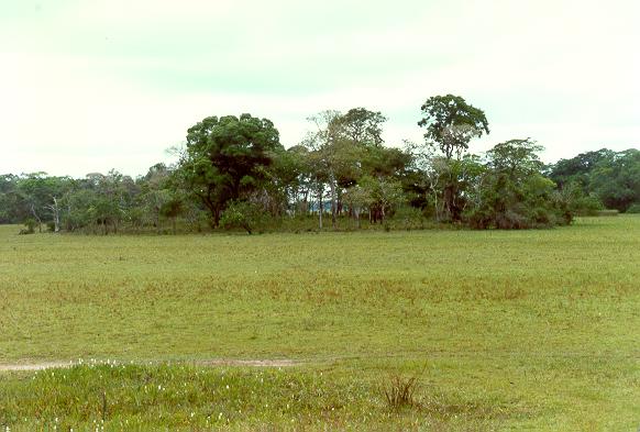
The sharpness of the campo/cerrado boundary has been documented by Eiten (1975). Within 1 m, or even 0.5 m, the change from the shrubs and low trees of the cerrado to the grassy layer without woody plants of the campo is complete. The reason for this abrupt change appears to be that the cerrado plants cannot establish themselves from seed in continually wet soil. In general, the campo occupies a site with a lower and more fluctuating water table, whereas the cerrado occupies the higher ground, where the soil seldom if ever remains saturated. In almost all cases, the cerrado stops suddenly at the edge of the campo, apparently due to the competition between the two vegetation types as whole plant communities. Cerrado species tolerant of waterlogging are able to grow in open campos in places where the soil level is only a few centimeters higher than elsewhere. The observation that larger islands on Pantanal landscape are thickly clothed with cerrado vegetation confirms that groundwater level exerts a precise control on the cerrado/campo boundary.
In the Pantanal, the main trend of vegetational variation is highly
correlated with soil moisture and topography. The patent lack of trees in the wet
campos is striking, particularly since a wide range of woody species successfully colonizes
both the interfluves, which are drier than the campos, and the stream sides
(riparian areas, or gallery forests) which are wetter. The absence of tall,
woody species from areas
which are intermediate in their physical characteristics is attributed to the fluctuating
nature of the water table and associated soil moisture. Thus, trees are able to tolerate both
permanently wet (gallery forest) and moist-to-dry (cerrado) environmental conditions, but
not an extreme alternation of saturation and desiccation
(Cole, 1960). Areas subject to
the latter are successfully colonized by the grassy elements
(see video:
C. The hammocks of South Florida
Vegetated earthmounds, conditioned as they are by local climate, hydrology, and geomorphology, occur in many parts of the world and are referred to by different names. For instance, the term hammock is used in the southeastern United States to refer to a stands of trees, usually hardwood, that forms an ecological island in a contrasting ecosystem. Hammocks grow on elevated areas, often just a few inches high, surrounded by wetlands that are too wet to support them.
In the Everglades swamp of South Florida (Fig. 61), the hammocks appear as teardrop-shaped islands, shaped by the
flow of water, in the middle of the slough (akin to airfoils in air navigation)
|
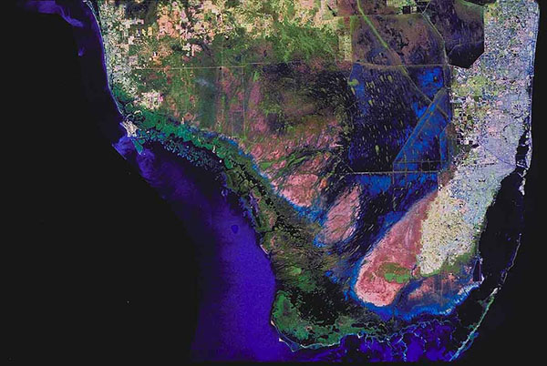
|
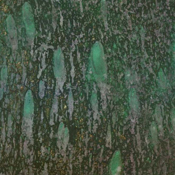
|
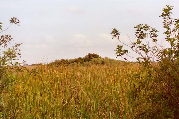
The genesis of the earthmounds appears to be either: (a) biotic, through the action of termites, which build mounds for habitat and survival; (b) abiotic, by differential sedimentation around the pioneer colony, to be interpreted in geologic time; or (c) mixed, when both termites and differential sedimentation join together for the same purpose (Ponce and Cunha, 1993 (Vegetated Earthmounds)). Figure 64 shows a small earthmound, most likely of biotic origin, in the floodplain of the Araguaia river, in Mato Grosso, Brazil.
|
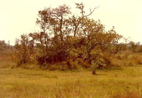
Clearly, the processes leading to the development of hammocks in the Everglades are the same processes responsible for the formation of capões and murundus in the Pantanal of Mato Grosso and other tropical ATTZ ecosystems. It is seen how geomorphology exerts a precise control on the boundary between the raised mounds, which are able to house woody vegetation, and the neighboring grassy fields, which are not.
D. The raised fields of the Llanos de Moxos, Bolivia
That geomorphology controls the boundary between grasses and other types of vegetation is further confirmed by the example of the raised fields of the Llanos de Mojos, in the western Beni, Bolivia (Denevan, 1966). The native Mojos people knew that their lands were too flat and subject to seasonal flooding. Throughout the years, they learned that the only way to properly feed themselves was to build the raised fields or camellones. These anthropogenic features of the landscape sought to causeway the floodwaters in order to keep portions of the land sufficiently dry throughout most, if not the entire year.
The number and aerial extent of these raised mounds, most of which still survive to this date, attest to the ingenuity and perseverance of the native peoples of the Llanos de Mojos. Denevan (op. cit.) has estimated a minimum of 100,000 drained fields occupying 15,000 acres spread unevenly over an area of 30,000 square miles in the western Beni (Figs. 65 and 66).
|
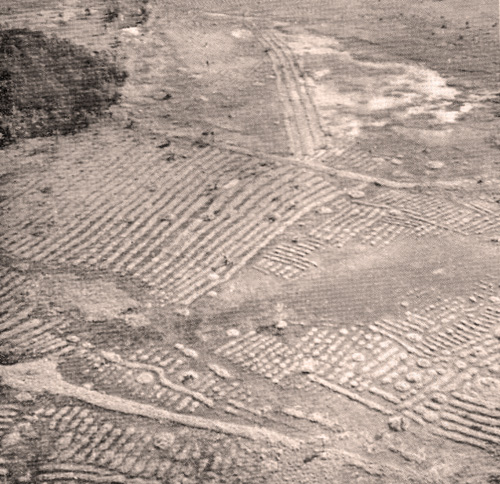
The rationale for the existence of the raised mounds invites thoughful consideration. In this connection, a knowledge of the nutrient balance may help clarify the matter (Delwiche, 1970). Export of nutrients is required in the management of artificial ecosystems. Nutrient export cannot proceed in the presence of effective nutrient cycling. In the absence of external inputs, a naturally denitrifying ecosystem will not work well for agriculture, because the nitrogen will be lost (returned to the atmosphere) and not be available for export.
In certain flood-pulse ecosystems, the combination of climate, geomorphology, and hydrology is such that it encourages denitrification. Alternating periods of aerobiosis and anaerobiosis in a natural ecosystem will lead to nitrification, followed by denitrification, and thus, the return of nitrogen to the atmosphere (Welch, 1982). Aerobiosis occurs during the dry period; anaerobiosis during the wet or flooding period, if the latter lasts long enough.
|
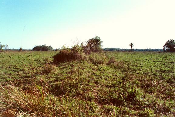
An annual flood pulse, with a sequence of dry and wet periods lasting approximately six months each, will have a tendency to close the nitrogen cycle. [Note that the rate of oxygen diffusion in water is 10,000 times smaller than that in air]. Anthropogenic nutrient export will be difficult under such conditions. The denitrifying ecosystems may be well suited for other uses, such as cattle grazing and wildlife habitat, but not for intensive agriculture.
In such flood-pulse ecosystems, the survival of woody vegetational communities hinges upon their symbiotic relationship with the earthmounds (Ponce, 2009a). Whether these mounds are built by nature or humans is inmaterial. Both mounds accomplish the same purpose: to provide an environment where vegetation other than grasses can survive and flourish.
E. Salinity balance in Tulare Lake Basin, California
The impact of geomorphology on ecohydrology is far-reaching, involving issues not only of water management but also of salt management. An interesting and extreme case of combined natural/anthropogenic salt sequestration is represented by Tulare Lake basin, near the southern tip of California's Central valley (Fig. 67).
Throughout geologic time, Tulare Lake has functioned as an endorheic basin most of the time, collecting its own local and regional runoff [Fig. 67 (a)]. However, during periods of extreme flood, runoff to Tulare Lake [shown in Fig. 67 (b) as the near circular darker green area north of the Kern river] would reverse direction and flow northward, towards the Kings and San Joaquin river valleys. From 1850 to 1878, the lake overflowed in 19 out of 29 years. Thus, historically, Tulare Lake functioned as a semi-endorheic basin, with occasional overflow to the north, which may have helped to keep the basin close to salt balance (Ponce, 2009b).
|
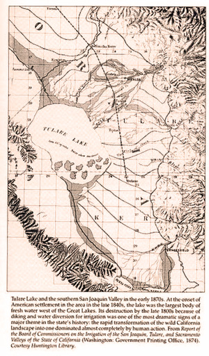
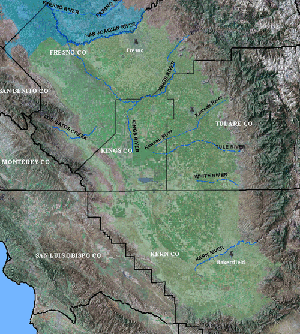
Since the 1890s, irrigation development in Tulare Lake and environs has resulted in the conversion of all runoff into vaporization.
While the intention (of irrigation) is to convert runoff into evapotranspiration, a significant portion of runoff is actually converted into
evaporation (from water-supply ponds and evaporation basins).
Every drop of water that precipitates in the basin is now captured in Tulare Lake basin;
therefore, not a single iota of salt is being allowed to leave the basin.
For the time being, the irrigation system works because the drainage system carries the salt brine away from the root zone,
handles it and accumulates it in evaporation basins (Fig. 68).
As the system continues to operate, the need for additional evaporation basins becomes apparent.
However, it is clear that the system is unsustainable, carrying with it the certainty of its eventual demise
(see video:
|
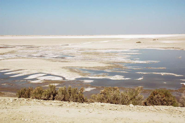
F. The vegetative lineaments of Tierra del Sol, California
A distinct characteristic of geology and geomorphology is their ability to affect the types and extent of vegetation on the surface of the Earth. Well known are the riparian corridors, driven by groundwater, and located along the sides of streams (Fig. 51). Lesser known are the vegetative lineaments, which occur in upland locations, in the absence of streams. When viewed from the air, the lineaments are seen as darker spots of approximate longitudinal orientation. They appear as such or are evident due to contrasts in terrain or ground cover on either side.
In Tierra del Sol, San Diego County, California, a substantial number of lineaments have been documented (Ponce, 2006). The region lies within the La Posta pluton, a deep-seated igneous intrusion within California's Peninsular Range batholith (Walawender et al., 1990). The lineaments are usually traced to faults, joints, or boundaries between stratigraphic formations. Groundwater seeps through these faults in cristalline rock (in this case, granodiorite) to sustain the longitudinal vegetational features.
Figure 69 shows a major lineament located east of
Tierra del Sol Creek, close to the bottom right-hand corner of the figure,
with a predominant northwest to southeast direction. Field inspection
showed that this lineament is composed of thick stands of red shank
(Adenostoma sparsifolium)
|
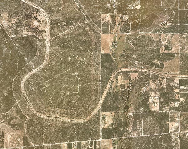
|
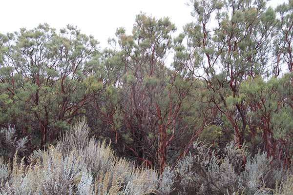
Figure 71 shows an infrared image (with vegetation showing up as red) covering approximately the same area as Fig. 69. Predictably, the major drainage courses (Tierra del Sol Creek and tributaries) feature riparian forests of coast live oak (shown as red dots in Fig. 71), which draw their moisture from the vadose and phreatic zones. The thick lineament in the bottom right-hand corner is located upland, i.e., it does not follow any clearly defined watercourse. Yet it is seen to consist of large shrubs (red shank) and trees (oak species) with a demonstrated water affinity.
|
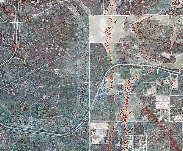
In Tierra del Sol, the substantial interaction between geology and geomorphology, on one side, and vegetational communities, on the other side, has been documented with field examples. Riparian communities and vegetative lineaments are but two of the links that make possible the study of ecohydroclimatology.
G. The recovery of Camp Creek, Oregon
Anthropogenic disturbances may produce geomorphological conditions which have ecohydroclimatological effects, as the experience of Camp Creek clearly shows (Ponce, 1990). Camp Creek, a tributary of the Crooked river, is located in Crook County, in semiarid central Oregon. It is about 64 km, in length, including its south, middle, and west forks. Before extensive settlement in the 1850s, the area drained by Camp Creek was a wet meadow, featuring predominantly grassy vegetation and a shallow water table maintained within root reach throughout the year. The grasses encouraged soil infiltration and made possible effective aquifer replenishment from year to year.
Around the late 1800s, overgrazing of the meadow led to increased quantities of surface runoff and incipient gully development. Under these conditions, severe floods triggered accelerated gully development which led to the incised channel (with almost vertical banks) which now cuts through the meadow (Fig. 72). Winegar (1977) has documented depths from 4.5 to 7.5 m and widths from 7.5 to 30 m.
|
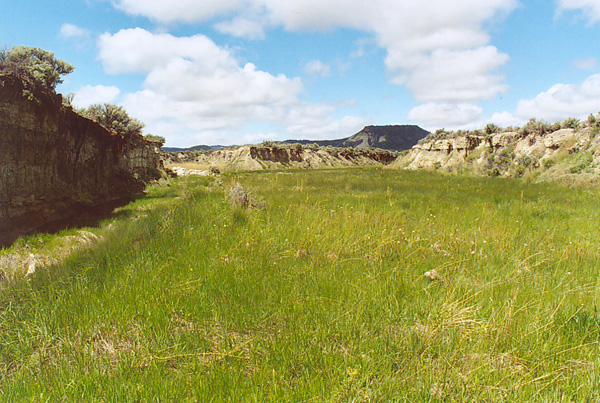
In time, inadequate aquifer replenishment led to the draining of the meadow and to the lowering of the water table to the point where it remained permanently out of reach of most herbaceous species. Over the several decades that ensued, the Camp creek valley underwent a change from a wet meadow to a predominantly dry area, with sagebrush (Artemisia sp.) taking over the former meadow.
About 1968, the Oregon Department of Fish and Wildlife and the Bureau of Land Management took bold steps to reverse the desertification of the Camp Creek valley. Approximately 6 km of the creek were fenced to exclude livestock (Elmore and Beschta, 1987). Over the years since the original fencing, exclusion of livestock has allowed the establishment of a healthy riparian area on the creek bed. This had led to a buildup of the streambed, a deeper and more stable low flow channel, and a reduction in sediment load, with net aggradation continuing to date.
Figure 73 shows two snapshots of the same reach of Camp Creek, taken in 1989 and 2004. Channel bed aggradation in the 15-year period is estimated at 0.6-0.9 m. At current rates of aggradation, full recovery of the Camp Creek meadow may be expected in 50 to 100 years.
The Camp Creek experience is an example of how enlightened management dealt effectively with anthropogenic disturbance to enable the recovery of a degraded watershed. The lesson to be learned is the different time scales of the geomorphic processes of erosion and deposition (sedimentation). While erosion may take a few events or seasons, deposition and full recovery is usually measured in decades.
|
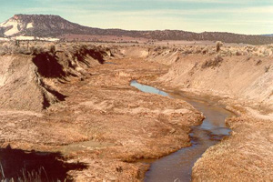
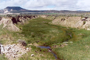
H. The restoration of Red Clover Creek, California
Red Clover Creek is a tributary of the North Fork Feather river, in Plumas County, California. Prior to the 1950s, Red Clover Creek was a relatively shallow stream with permanent baseflow supporting an excellent fishery. At about that time, federal programs were introduced to eliminate willows (phreatophytes) using aerial herbicide spraying. Additionally, over three hundred beaver were removed from the system. These actions, together with the longstanding effects of heavy grazing and a system of abandoned logging railroad grades in the valley, brought Red Clover Creek to the brink of collapse. The 1955 flood was the catalyst for the massive gully formation through the valley, which continued through most of the 1980s. Once the gully formed, the regional water table dropped, baseflow was all but lost, and erosion and sediment transport ensued.
After many years of enlightened management, Red Clover Creek has now returned to its former state: stable, self-sustaining, and with permanent baseflow. The restoration work began in 1985 with the construction of four loose-rock check dams. Several years later, a new technique was developed to use in place of the check dams. Called "pond and plug," it seeks to eliminate the gully through onsite excavation and fill, forcing the water level in the valley to rise to meet the historic remnant channels and floodplain.
In 2006 this technique was used on portions of Red Clover Creek downstream of the original check dam project. After treatment of 4.5 miles of stream channel, the project is in full recovery, as shown by the timed snapshots of Fig. 74. The restoration raised the water surface level up to 14 ft in some places (see video: The Story of Red Clover Creek).
|
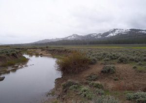
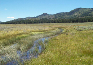
The experience of Red Clover Creek is an example of successful stream restoration following degradation by anthropogenic disturbance. Here again, it is shown how geomorphology interacts with hydrology and ecology to enable a return to productive ecosystem stability.
12. SUMMARY
|
|
Geomorphology serves as the link between ecology, hydrology, and climate, effectively underpinning the new field of ecohydroclimatology. Groundwater exists everywhere in the soil and rock mantle, deeper in arid regions and shallower in humid regions. Therefore, the distribution of plants of the Earth' surface is determined by:
Position along the climatic spectrum, from superarid to superhumid,
Depth to the water table, which determines whether the plants can avail themselves of moisture in the capillary fringe or the groundwater beneath it, and
The presence/absence of springs, which depends heavily on the local geology and geomorphology.
The importance of geomorphology is tempered by two factors:
Degree of dissection, which controls the timing and amount of runoff; and
Overall slope of the terrain, which determines the amount of runoff diffusion.
Several case studies are used to describe how knowledge of geomorphology is essential to the basic understanding of a broad class of processes in ecohydroclimatology.
REFERENCES
|
|
Alley, W. M., T. E. Reilly, and. O. E. Franke. 1999. Sustainability of groundwater resources. U.S. Geological Survey Circular 1186, Denver, Colorado, 79 p.
Arrhenius, S., 1896. On the influence of carbonic acid in the air upon the temperature of the ground. Philosophical Magazine and Journal of Science, Series 5, Vol. 41, No. 251, April, 237-276.
Balek, J. 1983. Hydrology and water resources in tropical regions. Developments in Water Science, 18, Elsevier Science Publishers BV, Amsterdam, Netherlands.
Beatty, S. W. 1984. Vegetation and soil patterns in Southern California chaparral communities. In B. Dell, editor, Medecos IV: Proceedings, 4th International Conference on Mediterranean Ecosystems, August 13-17, 1984, The Botany Department, University of Western Australia, Nedlands, Australia, 4-5.
Benton, G. S., R. T. Blackburn, and V. O. Snead. 1950. The role of the atmosphere in the hydrologic cycle. Eos Transactions, American Geophysical Union, Vol. 31, No. 1, 61-73.
Bredehoeft, J. 1997. Safe yield and the water budget myth. Editorial, Ground Water, Vol. 35, No. 6, page 29, November-December.
Budyko, M. I., and O. A. Drozdov. 1953. Characteristics of the moisture circulation in the atmosphere. Izv. Akad. Nauk. SSSR Ser. Geogr. Geofiz, 4, 5-14.
Chebotarev, I. I. 1955. Metamorphism of natural waters in the crust of weathering. Geochimica et Cosmochimica Acta, Vol. 8, 22-48, 137-170, 198-212.
Cloud, P., and A. Gibor. The oxygen cycle. Scientific American, Vol. 223, No. 3, September, 111-123.
Cole, M. 1960. Cerrado, caatinga, and pantanal: The distribution and origin of the savanna vegetation of Brazil. Geographical Journal, Vol. 129, 168-179.
Delwiche, C. C. 1970. The nitrogen cycle. Scientific American, Vol. 23, No. 3, September, 137-147.
Denevan, W. M. 1966. The aboriginal cultural geography of the Llanos de Mojos of Bolivia, Iberoamericana, 48, University of California Press, Berkeley and Los Angeles.
Eiten, G. 1975. The vegetation of the Serra do Roncador. Biotropica, 7, 112-135.
Elmore, W., and R. L. Beschta. 1987. Riparian Areas: Perceptions in Management, Rangelands, Vol. 9, No. 6, December, 260-265.
Entekhabi, D., I. Rodriguez-Iturbe, and R. L. Bras. 1992. Variability in large-scale water balance with land surface-atmosphere interactions. Journal of Climate, Vol. 5, 798-813.
Fuller, M. L. 1911. Protection of shallow wells in sandy deposits. U.S. Geological Survey Water Supply Paper No. 258, Washington, D.C.
Furley, P. A., and J. A. Ratter. 1988. Soil resources and plant communities of the Central Brazilian cerrado and their development. J. Biogeography, 15, 97-108.
Hayami, I. 1951. On the propagation of flood waves. Bulletin, Disaster Prevention Research Institute, No. 1, December.
Holdridge, L. R. 1947. Determinations of world plants formations from simple climatic data. Science, 105 (2727), 367-368.
Horton, R. E. 1933. The role of infiltration in the hydrologic cycle. Transactions, American Geophysical Union, Vol. 14, 446-460.
Hutchinson, G. E. 1970. The biosphere. Scientific American, Vol. 23, No. 3, September, 45-53.
Junk, W. J., P. B. Bailey, and R. E. Sparks. 1989. The flood-pulse concept in river-floodplain systems. Proceedings of the International Large River Symposium, Canadian Special Publication Fishing and Aquatic Sciences 106, 110-117.
Lettau, H., K. Lettau, and L. C. B. Molion. 1979. Amazonia's hydrologic cycle and the role of atmospheric recycling in assessing deforestation effects. Monthly Weather Review, Vol. 107, 227-237.
Lighthill, M. J., and G. B. Whitham. 1955. On kinematic waves: I. Flood movement in long rivers. Proceedings, Royal Society of London, Series A, 229, 281-316.
L'vovich, M. I. 1979. World water resources and their future. Translation from Russian by Raymond L. Nace, American Geophysical Union.
Meinzer, O. E. 1927. Plants as indicators of ground water. U.S. Geological Survey Water Supply Paper 577, Washington, D.C.
Ponce, V. M. 1989. Engineering hydrology: Principles and practices. Prentice Hall, Englewood Cliffs, New Jersey.
Ponce, V. M., and D. S. Lindquist. 1990. Management of baseflow augmentation: A review. Water Resources Bulletin, Vol. 26, No. 2, 259-268, April
Ponce, V. M., and C. N. da Cunha. 1993. Vegetated earthmounds in tropical savannas of Central Brazil: A synthesis; with special reference to the Pantanal of Mato Grosso. Journal of Biogeography, Vol. 20, 219-225.
Ponce, V. M., 1995. Hydrologic and environmental impact of the Parana-Paraguay Waterway on the Pantanal of Mato Grosso. Report, San Diego State University, San Diego, California, August.
Ponce, V. M., and A. V. Shetty. 1995a. A conceptual model of catchment balance: 1. Formulation and calibration. Journal of Hydrology, 173, 27-40.
Ponce, V. M., and A. V. Shetty. 1995b. A conceptual model of catchment balance: 2. Application to runoff and baseflow modeling. Journal of Hydrology, 173, 41-50.
Ponce, V. M., and R. H. Hawkins. 1996. Runoff curve number: Has it reached maturity? Journal of Hydrologic Engineering, ASCE, Vol. 1, No. 1, 11-19.
Ponce, V. M. 1996. Notes on my conversation with Vic Mockus. Online feature.
Ponce, V. M., A. K. Lohani, and P. T. Huston. 1997. Surface albedo and water resources: Hydroclimatological impact of human activities. Journal of Hydrologic Engineering, ASCE, Vol. 2, No. 4, October, 197-203.
Ponce, V. M., R. P. Pandey, and S. Ercan. 2000. Characterization of drought across climatic spectrum. Journal of Hydrologic Engineering, ASCE, Vol. 5, No. 2, April, 222-224.
Ponce, V. M., 2006. Impact of the proposed Campo landfill on the hydrology of the Tierra del Sol watershed. Online report.
Ponce, V. M., 2007. Sustainable yield of groundwater. Online report.
Ponce, V. M., 2008. Flood hydrology of the La Leche river, Lambayeque, Peru. Online report.
Ponce, V. M., 2009a. Nutrient balance under flood pulse. Online article.
Ponce, V. M., 2009b. Sustainable runoff for basin salt balance. Online article.
Ponce, V. M., 2011. The science of global warming. Online article.
Ponce, V. M., 2012. The salinity of groundwaters. Online article.
Ponce, V. M., 2013. Impacts of Soitec solar projects on Boulevard and surrounding communities, San Diego County, California. Online report.
Prance, G. T., and G. B. Schaller. 1982. Preliminary study of some vegetation types of the Pantanal, Mato Grosso, Brazil. Brittonia, 34, 228-251.
Prudic, D. E., and M. E. Herman. 1996. Ground-water flow and simulated effects of development in Paradise Valley, a basin tributary to the Humboldt River, in Humboldt County, Nevada. U.S. Geological Survey Professional Paper 1409-F.
Pulgar, I., J. Izco, and O. Jadan. 2010. Flora selecta de los pajonales de Loja, Ecuador. Ediciones Abya-Yala, Quito, Ecuador. 175 p.
Rivas-Martínez, S. 2007. Mapa de series, geoseries, y geopermaseries de vegetación de España. Memoria del mapa de vegetación potential de España. I. Itinera Geobotanica, Vol. 17, 5-435.
Salati, E., A. Dall'Olio, E. Matsui, and J. R. Gat. 1979. Recycling of water in the Amazon basin: An isotopic study. Water Resources Research, Vol. 15, No. 5, 1250-1258.
Salati, E., and P. B. Vose. 1984. Amazon basin: A system in equilibrium. Science, 225(4659), 129-138.
Schaller, G. B. 1983. Mammals and their biomass on a Brazilian ranch. Arquivos de Zoologia, Museu de Zoologia da Universidade de São Paulo, 31(1), 1-36.
Seddon, J. A. 1900. River hydraulics. Transactions, ASCE, Vol. XLIII, 179-243, June.
Smith, A. 1971. Mato Grosso: Last virgin land. Dutton, New York.
Sophocleous, M. (1997). Managing water resources systems: Why "safe yield" is not sustainable. Ground Water, Vol. 35, No.4, July-August, 561.
Stidd, C. K. 1975. Irrigation increases rainfall? Science, Vol. 188, 279-180.
Tricart, J. 1982. El Pantanal: Un ejemplo del impacto de la geomorfología sobre el medio ambiente. Geografía, 7(13-14), 37-50, São Paulo, Brazil.
Walawender, M. J., R. G. Gastil, J. P. Clinkenbeard, W. V. McCormick, B. G. Eastman, R. S. Wermicke, M. S., Wardlaw, S. H. Gunn, and B. M. Smith. (1990). Origin and evolution of the zoned La Posta-type plutons, eastern Peninsular Ranges batholith, Southern and Baja California. In "The Nature and Origin of Cordilleran Magmatism," J. Lawford Anderson, editor, Memoir 174, Geological Society of America, Boulder, Colorado.
Welch, E. B. 1982. Ecological effects of wastewater, Second Edition, Chapman and Hall, London.
Winegar, H. H. 1977. Camp Creek Channel Fencing--Plant, Wildlife, Soil and Water Response, Rangeman's Journal, Vol. 4 No. 1, February, 10-12.
World water balance and water resources of the Earth. (1978). USSR Committee for the International Hydrologic Decade, UNESCO, Paris.
| http://ponce.sdsu.edu/geomorphology.html |
|
170830 |